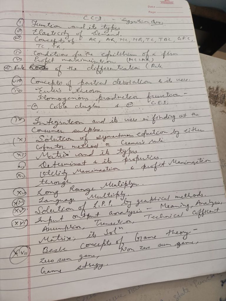
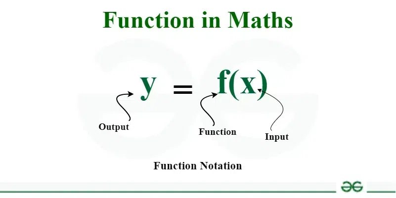
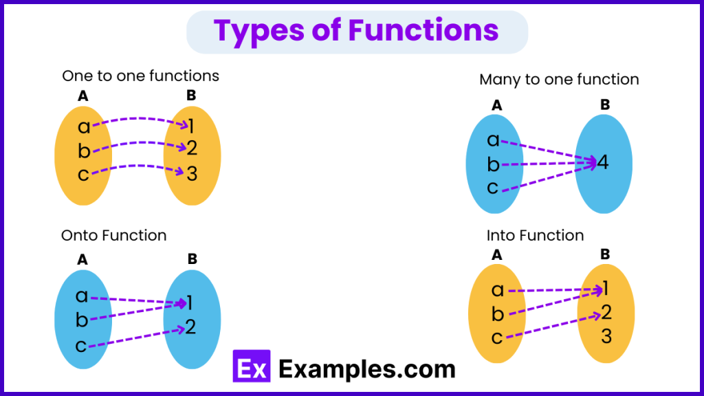
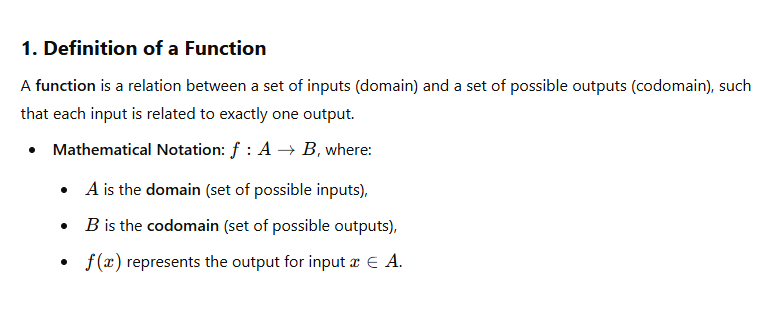
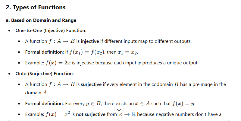
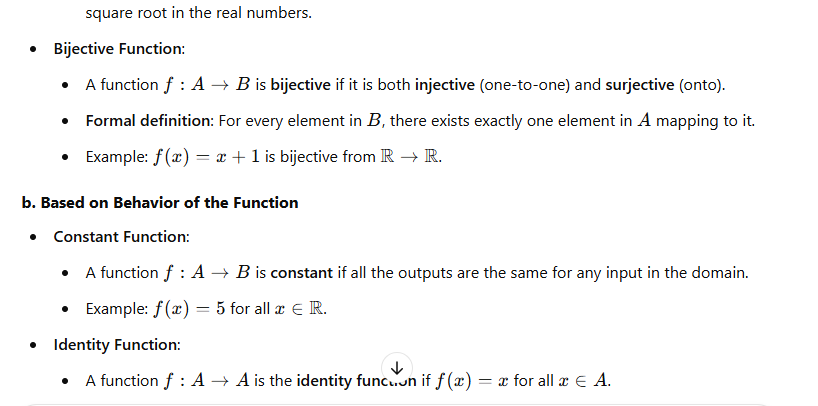
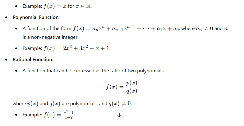
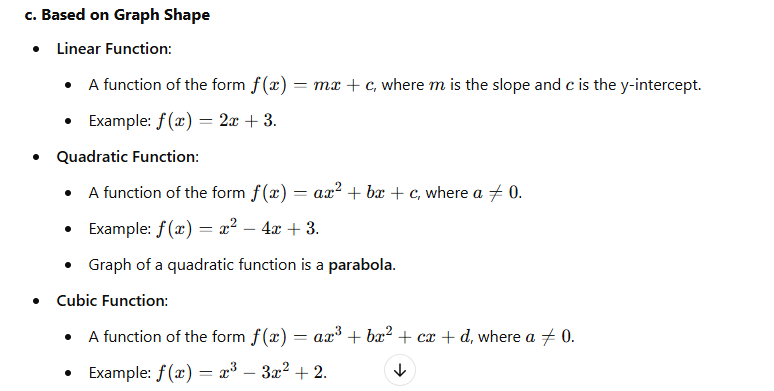
Q1. Function and its type
2. Elasticity of Demand
Here are concise exam notes on Elasticity of Demand, summarizing the key concepts, formulas, and applications.
Elasticity of Demand: Overview
- Elasticity of Demand measures the responsiveness of quantity demanded to changes in the price of a good or service.
- Formula for Price Elasticity of Demand (PED):
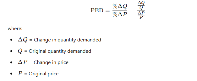
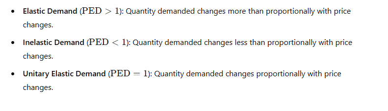
- Interpretation of PED:
Types of Elasticity of Demand
1. Price Elasticity of Demand (PED)
- Elastic Demand (PED > 1): A small price change causes a large change in quantity demanded.
- Example: Luxury goods or products with close substitutes (e.g., branded clothing).
- Inelastic Demand (PED < 1): A large price change causes only a small change in quantity demanded.
- Example: Necessities like salt, insulin, or gasoline.
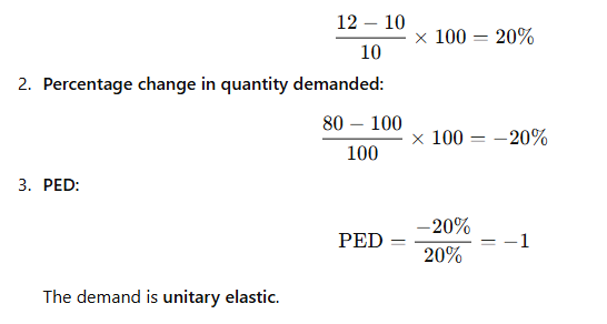
- Unitary Elastic Demand (PED = 1): A change in price results in a proportional change in quantity demanded.
- Example: A product where total revenue remains constant when price changes.
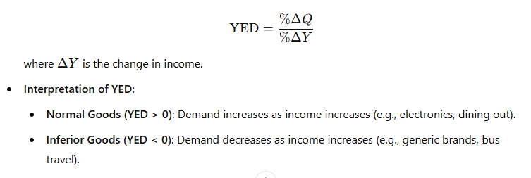
2. Income Elasticity of Demand (YED)
- Measures the responsiveness of demand to changes in income.
- Formula:
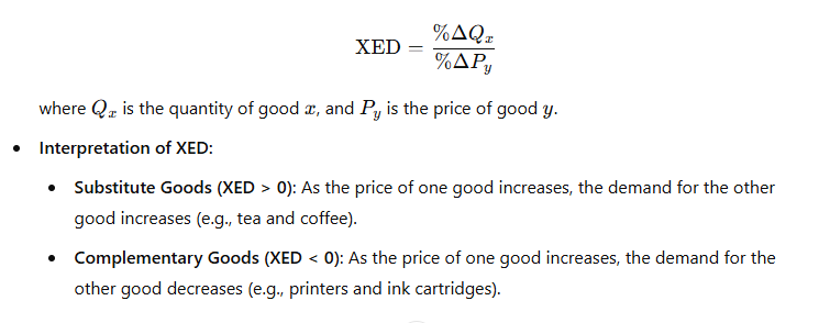
3. Cross-Price Elasticity of Demand (XED)
- Measures the responsiveness of demand for a good to changes in the price of another good.
- Formula:
Determinants of Price Elasticity of Demand
- Availability of Substitutes:
- More substitutes = more elastic demand.
- Example: If the price of one brand of cereal increases, consumers can easily switch to another brand.
- Necessities vs. Luxuries:
- Necessities tend to have inelastic demand (e.g., medicine).
- Luxuries tend to have elastic demand (e.g., designer handbags).
- Proportion of Income Spent on the Good:
- The higher the proportion of income spent on the good, the more elastic the demand.
- Example: A 10% increase in the price of a car will have a larger effect on demand than a 10% increase in the price of a pencil.
- Time Horizon:
- Demand tends to be more elastic in the long run than in the short run.
- Example: A sharp increase in fuel prices may not immediately decrease demand much, but over time, people might switch to more fuel-efficient cars.
- Brand Loyalty:
- Strong brand loyalty can make demand inelastic.
- Example: People may continue buying Apple products even if the prices increase because of their brand loyalty.
Applications of Elasticity
- Pricing Strategy:
- Elastic Demand: If demand is elastic, a decrease in price will increase total revenue, as the percentage increase in quantity demanded is larger than the percentage decrease in price.
- Inelastic Demand: If demand is inelastic, a price increase will increase total revenue, as the percentage decrease in quantity demanded is smaller than the percentage increase in price.
- Tax Incidence:
- Elastic Demand: Producers bear more of the tax burden because consumers can easily switch to alternatives.
- Inelastic Demand: Consumers bear more of the tax burden because they are less responsive to price changes.
- Total Revenue and Elasticity:
- Elastic Demand (PED > 1): Price decrease leads to higher total revenue.
- Inelastic Demand (PED < 1): Price increase leads to higher total revenue.
- Unitary Elastic (PED = 1): Total revenue remains unchanged when price changes.
Example Calculations
Example 1: Price Elasticity of Demand
Suppose the price of a good increases from $10 to $12, and the quantity demanded decreases from 100 units to 80 units. Calculate the PED.
- Percentage change in price:
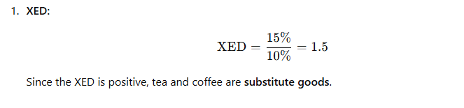
Example 2: Cross-Price Elasticity of Demand
Suppose the price of tea increases by 10%, and as a result, the demand for coffee increases by 15%. Calculate the XED between tea and coffee.
Summary of Key Points
- Price Elasticity of Demand (PED) measures responsiveness to price changes:
- Elastic: PED > 1
- Inelastic: PED < 1
- Unitary Elastic: PED = 1
- Income Elasticity of Demand (YED) measures responsiveness to changes in income:
- Normal Goods: YED > 0
- Inferior Goods: YED < 0
- Cross-Price Elasticity of Demand (XED) measures responsiveness to changes in the price of other goods:
- Substitutes: XED > 0
- Complements: XED < 0
These are the main points for Elasticity of Demand that will likely appear in exams. If you need more details or examples, feel free to ask!
3. Concept of AC, AR, MC, MR, TC, TBC,TFC, TVC, AFC, GFC, TC, TR
Here are concise exam notes covering the key concepts of AC, AR, MC, MR, TC, TBC, TFC, TVC, AFC, GFC, TC, and TR commonly used in economics:
1. Average Cost (AC)
- Definition: The total cost per unit of output.
- Formula:
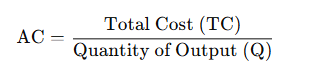
- Interpretation: It shows the cost of producing one additional unit of output. It includes both Fixed Costs (TFC) and Variable Costs (TVC).
2. Average Revenue (AR)
- Definition: The revenue per unit of output.
- Formula:

- Interpretation: For a firm in perfect competition, AR equals the price of the good. In other market structures, it may vary depending on pricing.
- In Perfect Competition:

3. Marginal Cost (MC)
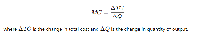
- Definition: The additional cost incurred by producing one more unit of output.
- Formula:
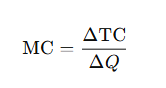
- Interpretation: It helps firms decide the optimal level of production. It usually rises after a certain level of production due to the law of diminishing returns.
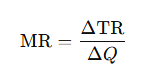
4. Marginal Revenue (MR)
- Definition: The additional revenue gained by selling one more unit of output.
- Formula:

5. Total Cost (TC)
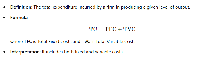
6. Total Variable Cost (TVC)
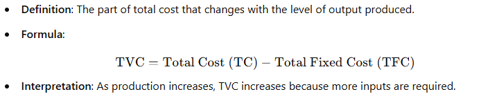
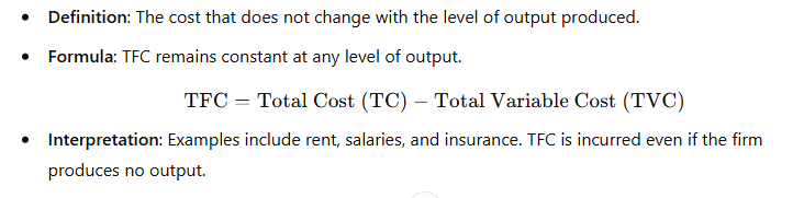
7. Total Fixed Cost (TFC)
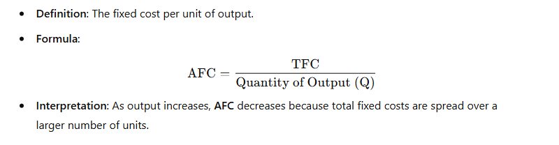
8. Average Fixed Cost (AFC)
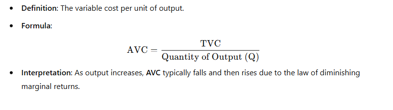
9. Average Variable Cost (AVC)
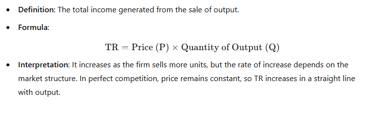
10. Total Revenue (TR)
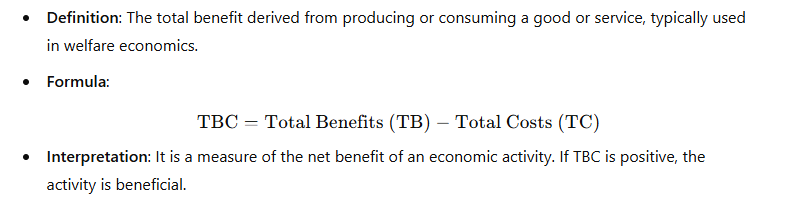
11. Total Benefit Cost (TBC) = Profit Samjho
12. Gross Fixed Cost (GFC)
- Definition: The total cost of fixed inputs or factors used in production.
- Interpretation: GFC is similar to TFC, representing the total cost of fixed inputs in the production process.
13. Relationship Between Cost and Revenue
- Profit Maximization Rule:
- A firm maximizes its profit when MC = MR.
- If MR > MC, the firm can increase output to increase profit.
- If MR < MC, the firm should reduce output to increase profit.
Key Concepts Summary Table
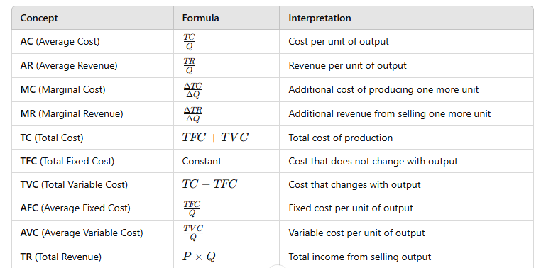

These notes should cover the main concepts related to cost, revenue, and profit in economics. These formulas and explanations are useful for understanding how businesses analyze production costs, pricing strategies, and overall profitability.
4. Condition for the equilibrium of a firm
Here are concise exam notes on the Conditions for the Equilibrium of a Firm in economics:
Condition for the Equilibrium of a Firm
A firm’s equilibrium occurs when it has no incentive to change its level of output or production. At equilibrium, the firm is maximizing its profit (or minimizing its loss) given the constraints it faces, such as costs and revenue.
1. Profit Maximization (Perfect Competition and Monopoly)
The key goal for a firm is to maximize profit, which occurs at the output level where the difference between total revenue (TR) and total cost (TC) is the highest.
- Profit Maximization Rule:
- A firm maximizes its profit when Marginal Revenue (MR) = Marginal Cost (MC).
- If MR > MC, the firm should increase output.
- If MR < MC, the firm should reduce output.
Mathematical Condition for Profit Maximization:
- MR = MC: This is the first condition for equilibrium. At this point, the firm is neither losing money nor missing out on any potential profit.
2. Marginal Cost and Marginal Revenue in Different Market Structures
- Perfect Competition: In perfect competition, a firm is a price taker. This means the price remains constant for the firm, and MR = Price (P). In equilibrium, MC = P.
- Monopoly: A monopoly is a price maker. The firm sets its own price. In this case, the firm maximizes profit by setting MR = MC, where the marginal revenue is less than the price due to the downward-sloping demand curve.
- Monopolistic Competition: Similar to a monopoly, firms have some control over price. They maximize profit where MR = MC, but they may not necessarily achieve productive or allocative efficiency.
- Oligopoly: The equilibrium condition of MR = MC holds, but due to strategic interactions between firms, the equilibrium might be more complex.
3. Second-Order Condition for Maximum Profit
While MR = MC ensures the firm is at an optimum output, it does not guarantee that this output level maximizes profit. The second-order condition checks whether the output level corresponds to a maximum rather than a minimum.
- Second-Order Condition for Maximum Profit: To confirm the firm is at a maximum profit and not a loss-minimizing point:
4. Conditions for the Long-Run Equilibrium in Perfect Competition
In the long run, a firm in perfect competition will only make normal profit (zero economic profit), meaning that it earns just enough to cover its opportunity costs. The following conditions apply:
- P = MC = AC (Average Cost):
- In the long run, the price equals both marginal cost and average cost. The firm earns zero economic profit, which means that Total Revenue (TR) = Total Cost (TC).
- No Incentive to Enter or Exit the Market:
- In long-run equilibrium, firms will enter or exit the market based on profitability. If firms are earning economic profits, new firms will enter the market, increasing supply and driving the price down until profits are eliminated. If firms are incurring losses, some will exit the market, reducing supply and driving the price up until firms are making normal profit again.
- Allocative Efficiency (P = MC):
- The firm is producing the quantity of output where the price consumers are willing to pay equals the marginal cost of production, reflecting an efficient allocation of resources.
- Productive Efficiency (P = AC):
- The firm is producing at the minimum point of its average cost curve, indicating that it is using the least cost method of production.
5. Conditions for Equilibrium in Monopoly
- Profit Maximization:
- Like any firm, a monopolist maximizes profit where MR = MC.
- Price Setting:
- The monopolist chooses the price that corresponds to the quantity where MR = MC on the demand curve. Since the monopolist is the sole seller, it has the ability to set the price above marginal cost.
- Second-Order Condition:
- The monopolist’s MR curve should be downward sloping, and the MC curve should intersect it from below to confirm that the point where MR = MC is a maximum profit point.
6. Conditions for Equilibrium in Monopolistic Competition
- Profit Maximization:
- As with other firms, a firm in monopolistic competition maximizes profit where MR = MC.
- Normal Profit in the Long Run:
- In the long run, firms in monopolistic competition earn only normal profit due to entry and exit of firms.
- P = AC in the long-run equilibrium, meaning firms earn zero economic profit.
- Product Differentiation:
- Unlike in perfect competition, firms in monopolistic competition sell differentiated products, meaning that each firm faces a downward-sloping demand curve.
7. Short-Run Equilibrium vs. Long-Run Equilibrium
- Short-Run Equilibrium:
- In the short run, a firm may earn economic profits or incur losses. The condition for equilibrium is still MR = MC, but the firm may not necessarily earn zero economic profit.
- Long-Run Equilibrium:
- In the long run, firms enter and exit the market, adjusting the price and quantity until economic profit is zero. The firm’s equilibrium condition is P = MC = AC in perfect competition, which leads to normal profit.
Summary of Key Equilibrium Conditions
- Perfect Competition:
- P = MC = AC (Long-run equilibrium condition).
- Profit Maximization: MR = MC.
- Monopoly:
- MR = MC (Profit Maximization).
- Price is set above MC due to the firm’s market power.
- Monopolistic Competition:
- MR = MC (Profit Maximization).
- P = AC in the long run (Normal profit).
- Oligopoly:
- MR = MC (Profit Maximization), but firms may take into account competitors’ actions (strategic behavior).
- Equilibrium may involve Price Rigidity and Non-Price Competition.
These are the key conditions for the equilibrium of a firm in different market structures. The conditions help understand how firms behave in various competitive environments and the strategies they use to maximize profits or minimize losses.
5. Profit maximization MC=MR
Here are concise exam notes on Profit Maximization and the MC = MR rule in economics:
Profit Maximization and the MC = MR Rule
Profit maximization is the primary goal of firms in both the short run and long run. A firm maximizes its profit when it chooses the optimal level of output at which the difference between total revenue (TR) and total cost (TC) is the greatest.
Key Concept: Marginal Revenue (MR) and Marginal Cost (MC)
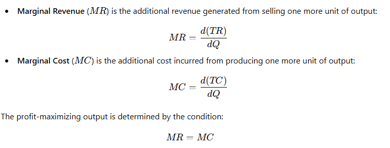
- Marginal Revenue (MR): The additional revenue gained by selling one more unit of output.
- Formula:
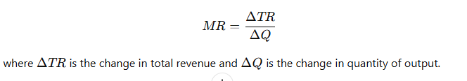
- Marginal Cost (MC): The additional cost incurred by producing one more unit of output.
- Formula:
Profit Maximization Rule: MC = MR
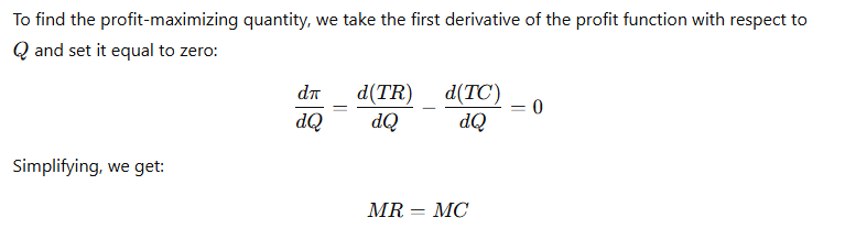
- The profit-maximizing level of output occurs where: MR=MCMR = MC This means that the firm will maximize its profit by producing the level of output where the marginal cost (MC) of producing an additional unit equals the marginal revenue (MR) gained from selling that unit.
Reason for the MC = MR Rule
- If MR > MC:
- The firm can increase profit by producing more units because the additional revenue from selling an extra unit exceeds the cost of producing that unit.
- The firm should expand production.
- If MR < MC:
- The firm is producing too much, and the cost of producing an additional unit exceeds the revenue it generates. The firm should reduce production.
- If MR = MC:
- The firm is at the profit-maximizing level of output. The cost of producing one more unit is exactly equal to the revenue gained from selling that unit.
First-Order Condition for Profit Maximization
- The first-order condition for profit maximization is that the firm sets its output level where MR = MC.
- At this point, the firm’s profit is maximized because the additional cost of producing one more unit is exactly equal to the additional revenue it would gain from that unit.
- The firm’s total profit can be calculated as the difference between total revenue (TR) and total cost (TC).
Second-Order Condition for Maximum Profit
- While MR = MC gives the optimal output, it does not guarantee that this output level corresponds to a maximum profit. The second-order condition ensures that the point where MR = MC corresponds to a maximum profit and not a loss-minimizing point.
Profit Maximization in Different Market Structures
- Perfect Competition:
- In perfect competition, MR = P (Price is constant for each firm since the firm is a price taker).
- Profit Maximization Condition: P=MCP = MC Firms will produce the quantity of output at which Price = Marginal Cost. In the long run, firms will earn normal profit, meaning P = AC.
- Monopoly:
- In a monopoly, the firm sets the price, and its demand curve is downward-sloping. The firm maximizes profit where MR = MC.
- Since the monopolist faces a downward-sloping demand curve, MR < P. The monopolist will produce less output and charge a higher price than in perfect competition, leading to economic profit.
- Monopolistic Competition:
- In monopolistic competition, firms also maximize profit where MR = MC, but they face a downward-sloping demand curve due to product differentiation.
- In the long run, firms earn normal profit, and the condition for equilibrium is P = AC, where P > MC.
- Oligopoly:
- In an oligopoly, firms may have some degree of pricing power and face interdependent behavior from other firms.
- Profit maximization occurs at the point where MR = MC, but the firm’s strategy is influenced by how other firms in the industry react to price changes or output changes (e.g., through price leadership or game theory).
Graphical Representation of Profit Maximization
- Perfect Competition:
- In perfect competition, the firm’s MR curve is horizontal at the price level, and the firm produces where P = MC.
- Monopoly:
- In a monopoly, the MR curve is downward sloping and lies below the demand curve. The monopolist maximizes profit by setting output where MR = MC and charging the price corresponding to that output on the demand curve.
Relation Between Marginal Revenue, Marginal Cost, and Profit
- Profit = Total Revenue (TR) – Total Cost (TC)
- Total Revenue (TR) increases as more units are sold, but it does so at a decreasing rate when demand is elastic.
- Total Cost (TC) increases as output increases, but the rate of increase in costs depends on the firm’s production efficiency.
- At profit-maximizing output:
- The increase in total revenue (MR) exactly equals the increase in total cost (MC), meaning the firm is not losing money by producing more units or sacrificing revenue by producing fewer units.
Summary of Key Points
- Profit Maximization Rule: The firm maximizes profit when MR = MC.
- First Condition for Profit Maximization: MR = MC. This ensures that the firm is producing the optimal quantity of output.
- Second Condition for Maximum Profit: The firm should ensure that MC is increasing at the point where it intersects MR.
- Perfect Competition: In the long run, firms earn normal profit and produce where P = MC.
- Monopoly: A monopolist maximizes profit where MR = MC, but P > MC.
- Monopolistic Competition and Oligopoly: Firms also maximize profit where MR = MC, but face different pricing behaviors and market structures.
These notes summarize the profit maximization rule and how MC = MR applies across different market structures. Let me know if you’d like additional clarification or examples!
6. Rule of Differentiation
Here are concise exam notes on the Rules of Differentiation in calculus, which are widely used in economics for analyzing functions like cost, revenue, and profit:
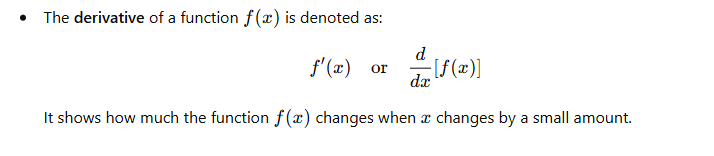
Differentiation: Basic Concept
- Differentiation is the process of finding the derivative of a function, which represents the rate of change of the function with respect to a variable. In economics, this is often used to determine things like marginal cost, marginal revenue, and elasticity.
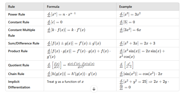
Basic Rules of Differentiation
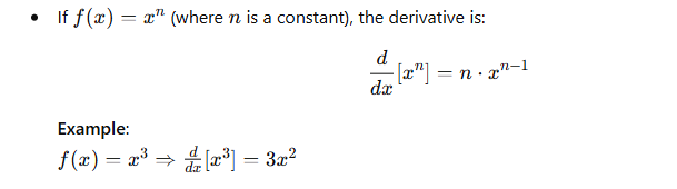
1. Power Rule
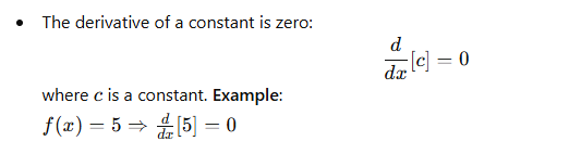
2. Constant Rule
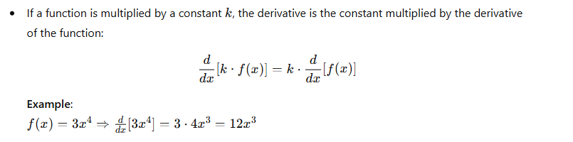
3. Constant Multiple Rule
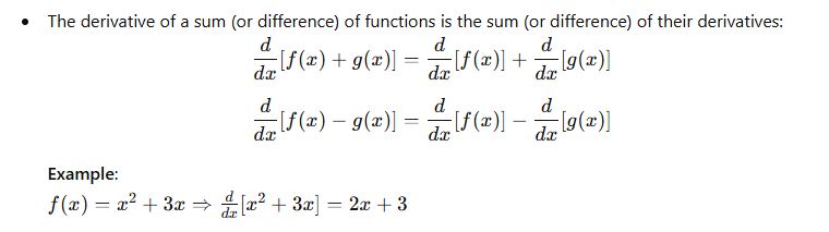
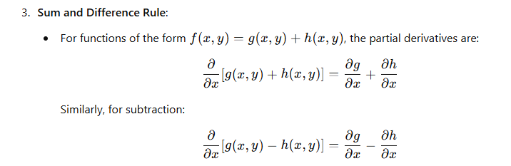
4. Sum and Difference Rule
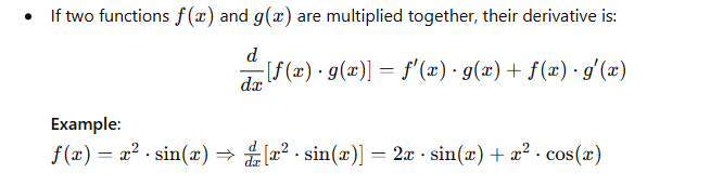
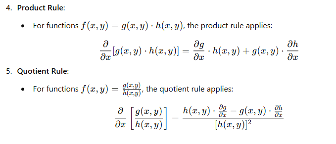
5. Product Rule
6. Quotient Rule
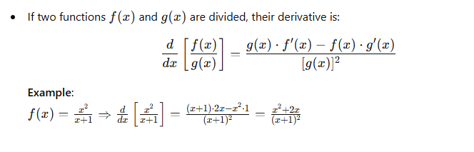
Advanced Differentiation Rules
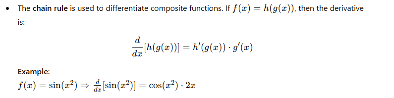
7. Chain Rule
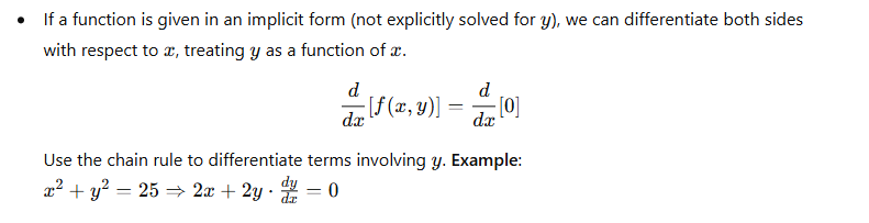
8. Implicit Differentiation
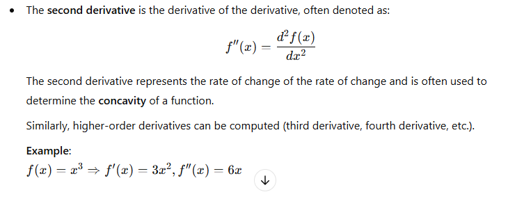
9. Higher-Order Derivatives
Common Economic Functions and Their Derivatives
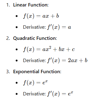
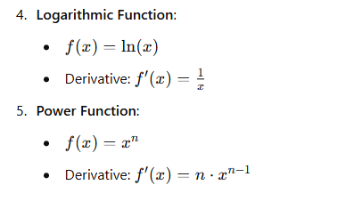
Applications of Differentiation in Economics
3. Profit Maximization:
- Firms use differentiation to find the level of output at which marginal cost (MC) equals marginal revenue (MR) to maximize profit.
Summary of Key Differentiation Rules
These rules and applications of differentiation are foundational for understanding changes in economic variables such as costs, revenue, and profit. Let me know if you’d like further clarification!
7. Concept of Partial Differentiation and its use
Here are exam notes on the Concept of Partial Differentiation and its uses, which are essential for understanding multivariable functions and their applications in economics:
Concept of Partial Differentiation
Partial differentiation is a technique used to differentiate functions of multiple variables. Unlike ordinary differentiation, where a function depends on one variable, partial differentiation involves finding the derivative of a function with respect to one variable while treating other variables as constants.
Definition of Partial Derivative
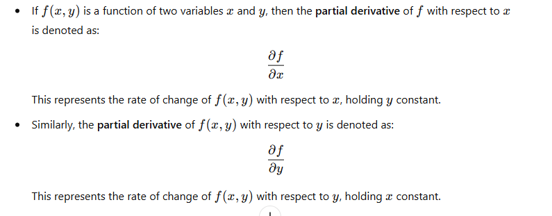
Notation
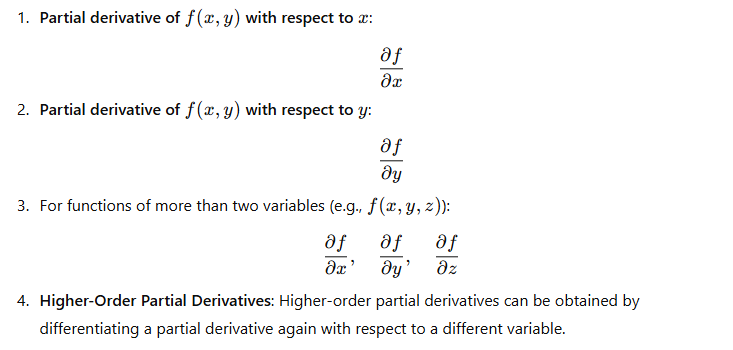
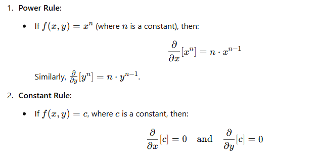
Basic Rules of Partial Differentiation
Applications of Partial Differentiation in Economics
Partial differentiation plays a crucial role in economics, especially when dealing with multivariable functions such as production functions, cost functions, and utility functions. It helps to analyze how one variable affects the outcome when others are held constant.
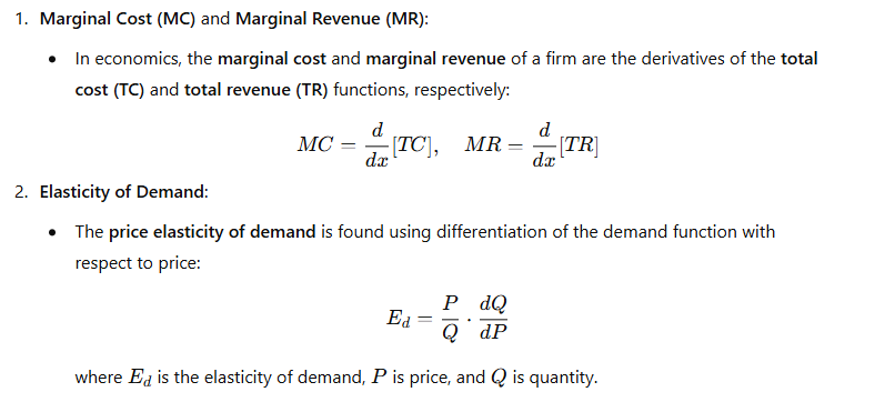
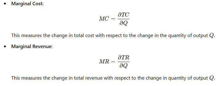
1. Marginal Analysis (Marginal Cost, Marginal Revenue)
- Marginal cost (MC) and marginal revenue (MR) can be derived from total cost (TC) and total revenue (TR) functions using partial differentiation:
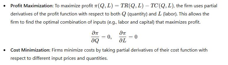
2. Optimization in Multivariable Functions
3. Elasticity of Substitution

4. Utility Maximization in Consumer Theory
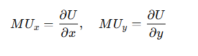
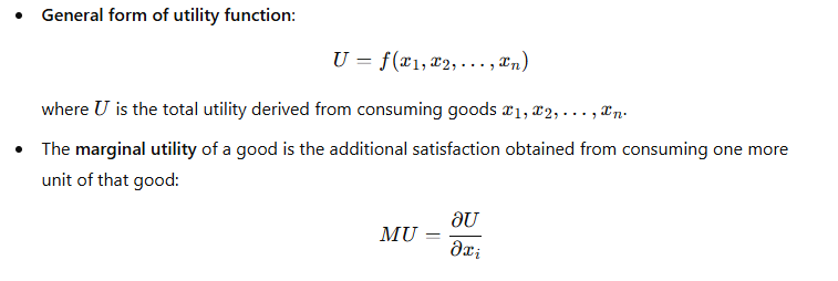
- Consumers maximize utility subject to their budget constraint. If the utility function U(x,y)U(x, y) depends on two goods xx and yy, the marginal utility of each good is given by the partial derivative of the utility function:
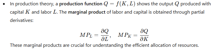
5. Production Function and Isoquants
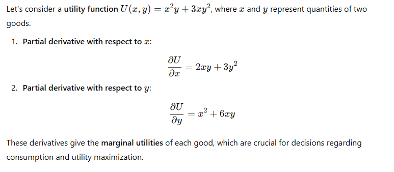
Example of Partial Differentiation
Summary
- Partial differentiation is used to find how a function changes with respect to one variable while holding others constant.
- Partial derivatives are crucial in multivariable optimization, such as profit maximization, cost minimization, and utility maximization in economics.
- Important rules of partial differentiation include the power rule, product rule, and quotient rule.
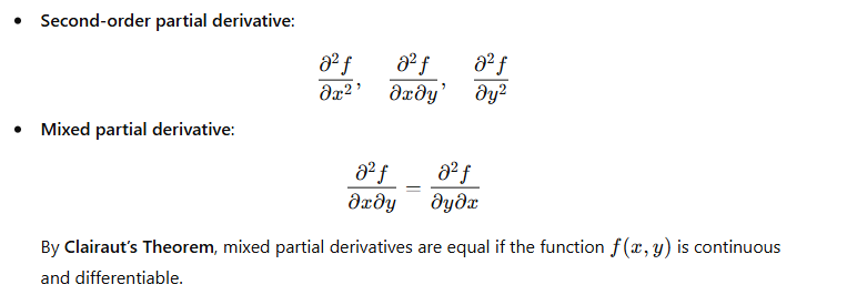
- Higher-order partial derivatives and mixed partials help understand the curvature and interactions between variables.
- Applications are seen in various fields of economics like marginal analysis, elasticity, production functions, and consumer theory.
These concepts form the foundation for analyzing complex economic models involving multiple variables. Let me know if you need further examples or clarifications!
8. Euler’s Theorem, Homogeneous Production Function, Cobb Douglas and CES
Here are exam notes on Euler’s Theorem, Homogeneous Production Function, Cobb-Douglas Production Function, and CES (Constant Elasticity of Substitution) Production Function:
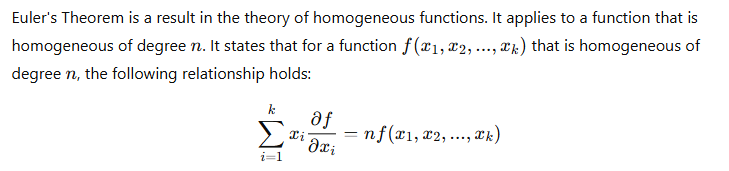
Euler’s Theorem:
Key Points:
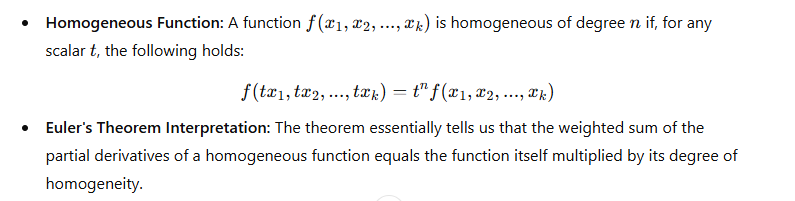
Application in Economics:
In production theory, if a production function is homogeneous of degree 1 (i.e., it exhibits constant returns to scale), Euler’s Theorem implies that the total value of output is equal to the total cost of inputs.
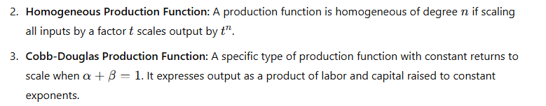
Homogeneous Production Function:
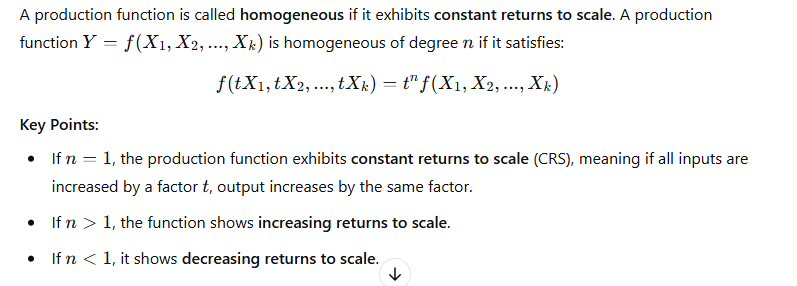
Example:

Cobb-Douglas Production Function:
The Cobb-Douglas production function is a widely used functional form in economics, which describes the relationship between two or more inputs and output. The general form of the Cobb-Douglas production function is:
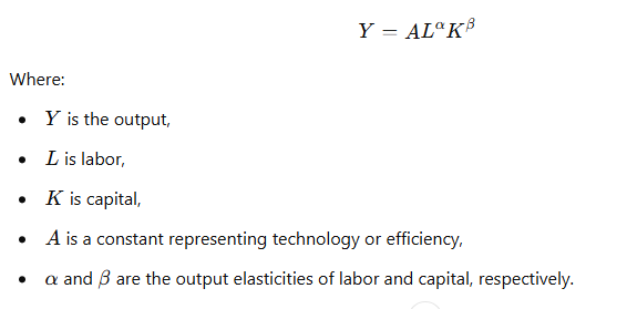
Key Points:
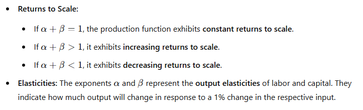
Example:
CES (Constant Elasticity of Substitution) Production Function:
The CES production function is a more general form of the production function that allows for a constant elasticity of substitution between inputs. The general form is:
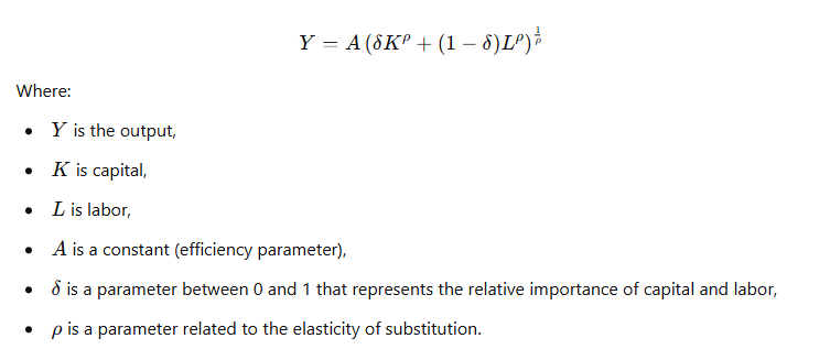
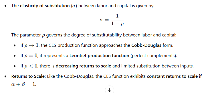
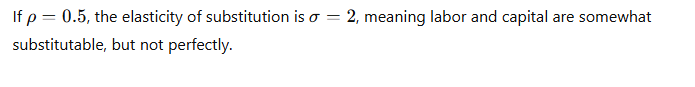
Key Points:
Example:
Summary of Key Concepts:
- Euler’s Theorem: Relates to homogeneous functions, stating that the weighted sum of partial derivatives equals the function scaled by its degree of homogeneity.
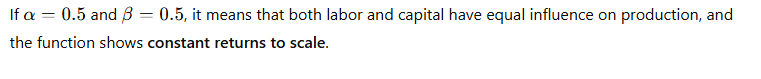
4. CES Production Function: A general form of production function allowing for a constant elasticity of substitution between inputs. It generalizes the Cobb-Douglas function and can model different degrees of substitutability between labor and capital.
9. Integration and its use in finding at the consumer surplus
Here are the exam notes on Integration and its use in finding Consumer Surplus:
1. Integration in Economics
Integration is a mathematical operation that is often used to find the area under curves, and it plays an important role in various economic calculations. It is particularly useful for calculating areas that represent consumer and producer surplus, total revenue, and other economic measures.
Basic Concept of Integration:
- Integration is the reverse of differentiation, and it is used to calculate the total accumulated value of a function over a range. In economics, it often refers to finding the area under a curve.

- Indefinite Integral: When no limits are provided, it is called the indefinite integral, which gives a general formula.
- Definite Integral: When limits are given, it is called the definite integral, and it represents the exact area under the curve between those limits.
2. Consumer Surplus
Consumer surplus represents the benefit consumers receive when they are able to purchase a product for a price lower than the maximum price they are willing to pay. It is the difference between what consumers are willing to pay (demand curve) and what they actually pay (market price).
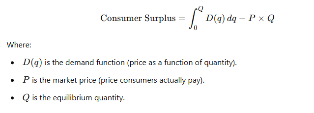
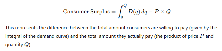
Consumer Surplus Formula:
Consumer surplus is represented graphically as the area between the demand curve and the price line up to the quantity purchased. Mathematically, it can be calculated using integration.
Graphical Representation:
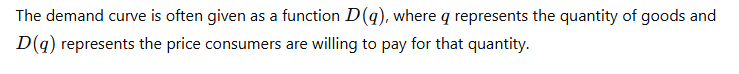
- The demand curve shows the price consumers are willing to pay for each unit of a good.
- The market price is where the supply and demand curves intersect (or the price consumers actually pay).
- Consumer surplus is the area between the demand curve and the market price, up to the equilibrium quantity.
3. Using Integration to Find Consumer Surplus
To calculate consumer surplus using integration, we need to:
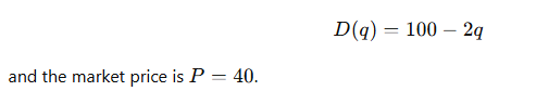
- Determine the demand curve: This function expresses the price consumers are willing to pay for each quantity of the good.
- Find the market price (P): This is the actual price consumers pay in the market.
- Find the equilibrium quantity (Q): This is the quantity at which the demand curve intersects the price line.
- Integrate the demand curve: This calculates the total value consumers would place on the good at different quantities.
- Subtract the total amount consumers actually pay: This gives us the net consumer surplus.
4. Steps for Finding Consumer Surplus Using Integration
Step 1: Set Up the Demand Curve
Step 2: Find the Market Price (P) and Equilibrium Quantity (Q)
The equilibrium price is typically given or determined by market forces, and it corresponds to the price at which the quantity demanded equals the quantity supplied.
Step 3: Set Up the Integral for Consumer Surplus
The consumer surplus is the area under the demand curve, from 0 to the equilibrium quantity QQ, minus the total amount spent by consumers:
Step 4: Solve the Integral and Subtract the Total Amount Paid

5. Example of Calculating Consumer Surplus Using Integration
Suppose the demand curve is:
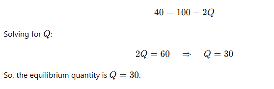
Step 1: Find the Equilibrium Quantity (Q)
Set the demand curve equal to the market price to find the equilibrium quantity Q:
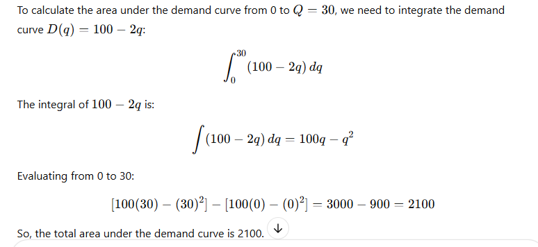
Step 2: Set Up the Integral for Consumer Surplus
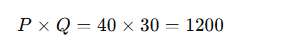
Step 3: Calculate the Total Amount Paid by Consumers
The total amount consumers actually pay is:
Step 4: Calculate Consumer Surplus
Finally, the consumer surplus is the area under the demand curve minus the total expenditure:
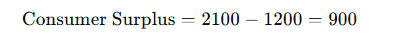
Thus, the consumer surplus is 900.
6. Graphical Interpretation of Consumer Surplus
Graphically, consumer surplus is represented by the area of the triangle formed between:
- The demand curve,
- The price line at the market price P, and
- The quantity axis (from 0 to Q).
This triangular area represents the net benefit to consumers from participating in the market.
7. Key Points to Remember:
- Integration is used to calculate areas under curves, which is essential in finding economic measures like consumer surplus.
- Consumer surplus is the difference between the total value consumers place on a good (represented by the area under the demand curve) and the amount they actually pay for it.
- The formula for consumer surplus involves integrating the demand curve and subtracting the total amount spent by consumers.
- Consumer Surplus = Area under demand curve from 0 to Q – Total amount spent by consumers.
These notes provide a comprehensive understanding of integration and its role in calculating consumer surplus, a central concept in microeconomics.
10. Solution of Simultaneous equation by Cofactor Method and Cramer’s rule
Exam Notes: Solution of Simultaneous Equations by Cofactor Method and Cramer’s Rule
1. Simultaneous Equations:
Simultaneous equations are a set of equations that share common variables. The solution to a system of simultaneous equations is the set of values for the variables that satisfy all equations simultaneously.
For example, a system of two equations in two variables x and y:
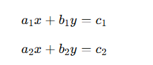
These can be solved using different methods, including Cofactor Method and Cramer’s Rule.
2. Cofactor Method:
The Cofactor Method is used to solve systems of linear equations. It is often used in conjunction with the determinant of a matrix.
Steps for Solving a System of Equations using Cofactor Method:
Given a system of n linear equations with n unknowns, written in matrix form as:
Step 1: Write the system in matrix form
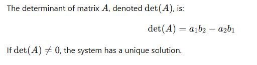
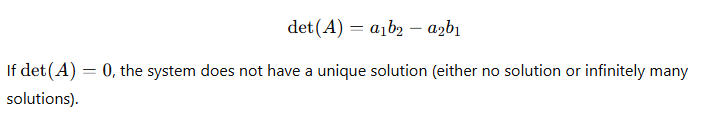
Step 2: Find the determinant of matrix AA
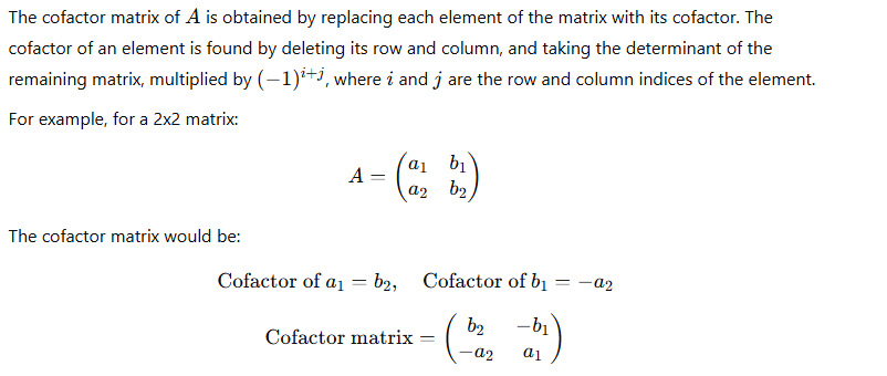
Step 3: Calculate the cofactor matrix
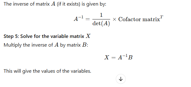
Step 4: Find the inverse of AA
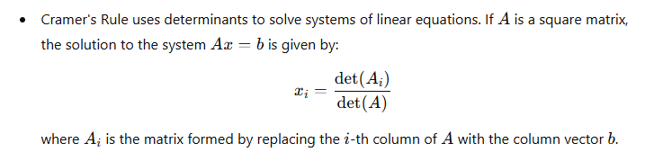
3. Cramer’s Rule:
Cramer’s Rule is another method used to solve a system of linear equations using determinants. It is applicable when the system of equations is square (i.e., the number of equations equals the number of unknowns) and the determinant of the coefficient matrix is non-zero.
Steps for Solving a System of Equations using Cramer’s Rule:
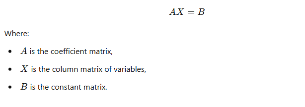
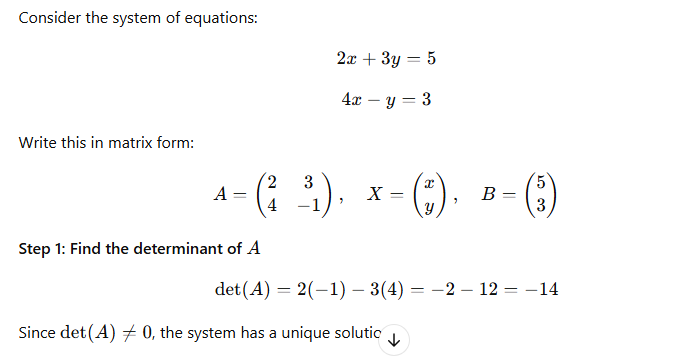
Given a system of n linear equations in n variables, written in matrix form AX=B, where:
- A is the coefficient matrix,
- X is the column matrix of variables,
- B is the constant matrix.
The solution to the system is found using Cramer’s Rule, which provides a formula for each variable in terms of determinants.
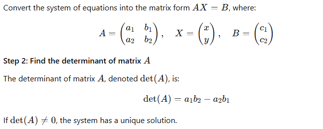
Step 1: Write the system in matrix form

Step 2: Find the determinant of matrix AA Calculate the determinant of the coefficient matrix AA:
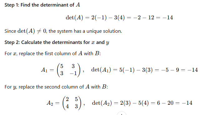
Step 3: Form matrices to find the variables
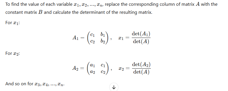
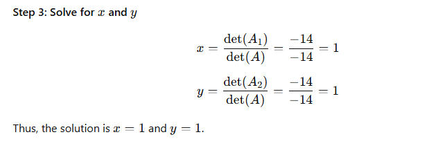
Step 4: Solve for the variables
After calculating the determinants for each modified matrix, solve for the variables.
4. Example Using Cramer’s Rule:
Key Points to Remember:
- Cofactor Method involves finding the determinant of the coefficient matrix, finding the cofactor matrix, and using the inverse of the matrix to solve for the variables.
- Cramer’s Rule uses the determinants of matrices formed by replacing columns of the coefficient matrix with the constant matrix to solve for the variables.
- Determinants play a crucial role in both methods, and a non-zero determinant indicates a unique solution.
These methods are applicable to square systems of linear equations (i.e., systems where the number of equations equals the number of unknowns).
11. Matrix and its Type
Exam Notes: Matrix and Its Types
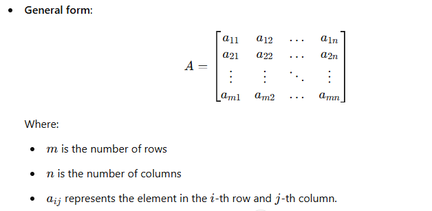
1. Matrix: Definition
A matrix is a rectangular arrangement of numbers, symbols, or expressions in rows and columns. It is usually enclosed within brackets.
2. Types of Matrices
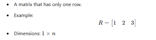
- Row Matrix:
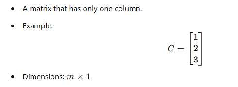
2. Column Matrix:
3. Square Matrix:
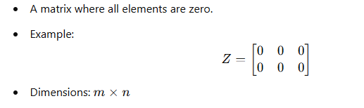
4. Zero Matrix (Null Matrix):
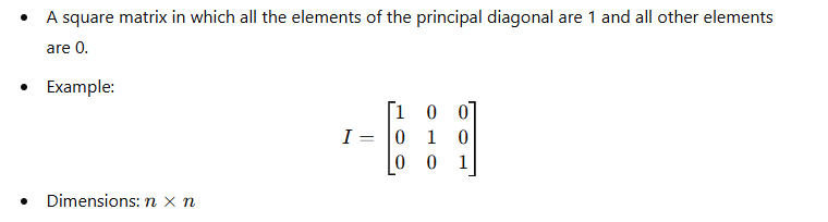
5. Identity Matrix:
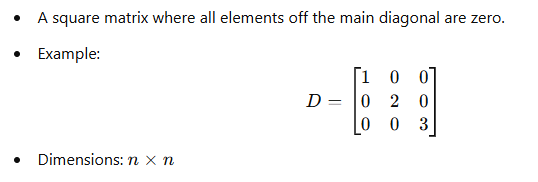
6. Diagonal Matrix:
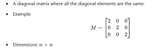
7. Scalar Matrix:
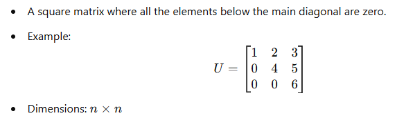
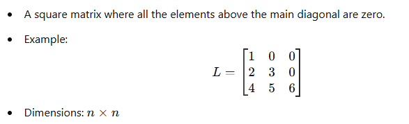
8. Upper Triangular Matrix:
9. Lower Triangular Matrix:
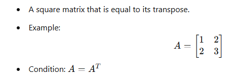
10. Symmetric Matrix:
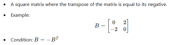
11. Skew-Symmetric Matrix:
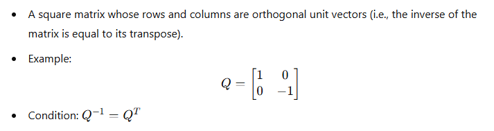
12. Orthogonal Matrix:
13. Sparse Matrix:
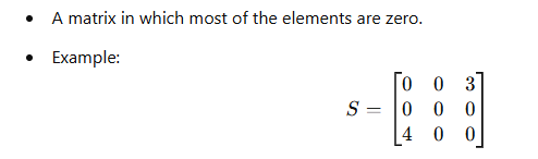
14. Dense Matrix:
- A matrix where most of the elements are non-zero.
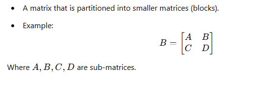
15. Block Matrix:
3. Matrix Operations (Basic Overview)
- Addition: Matrices can be added if they have the same dimensions.
- Scalar Multiplication: Each element of the matrix is multiplied by a scalar.
- Matrix Multiplication: The number of columns in the first matrix must be equal to the number of rows in the second matrix.
- Transpose: The rows and columns of a matrix are swapped.
- Inverse: A matrix has an inverse if and only if it is square and its determinant is non-zero.
4. Special Properties
- Trace of a Matrix: The sum of the diagonal elements of a square matrix.
- Determinant: A scalar value that is computed from the elements of a square matrix.
- Rank: The number of linearly independent rows or columns in a matrix.
These notes cover the key types and operations related to matrices. Be sure to focus on matrix properties and operations as they form the foundation for many linear algebra problems!
12. Determinant and its properties
Exam Notes: Determinants and Its Properties
1. Determinant: Definition
The determinant of a square matrix is a special scalar value that is computed from its elements and reflects certain properties of the matrix, such as whether the matrix is invertible (non-zero determinant) or singular (zero determinant).
2. Properties of Determinants
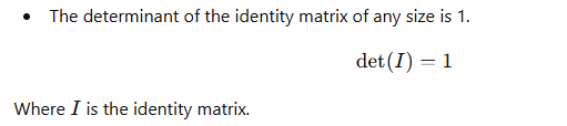
- Determinant of the Identity Matrix:
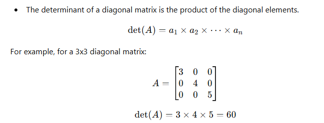
- Determinant of a Diagonal Matrix:
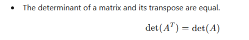
- Determinant of a Transpose Matrix:
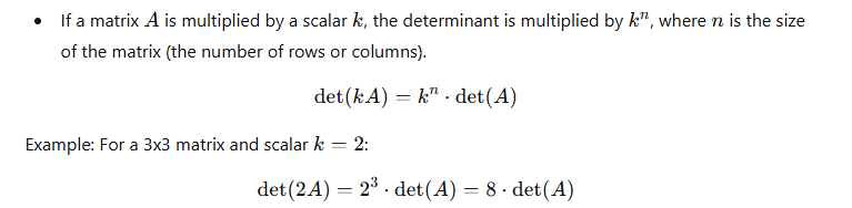
- Determinant of a Scalar Multiple of a Matrix:
- Determinant of a Product of Matrices:

- Effect of Row Operations on Determinants:
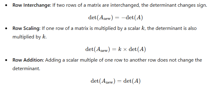
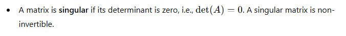
- Singular Matrix:
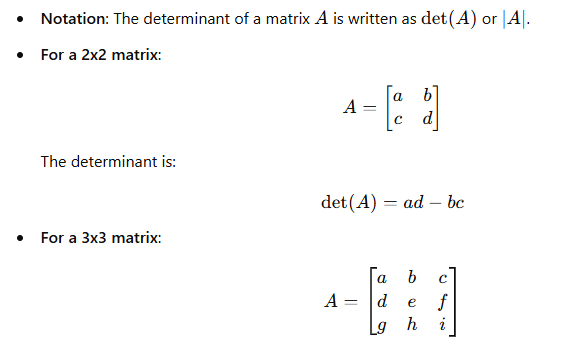
- Determinant of a 2×2 Matrix:

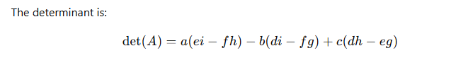
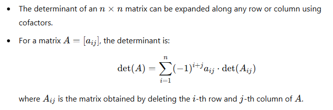
- Cofactor Expansion (Laplace Expansion):
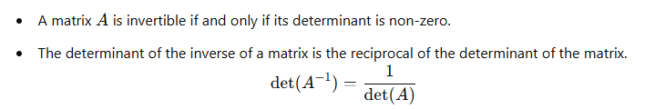
- Determinant and Inverses:
- Determinant of a Block Matrix:
- For a block matrix, the determinant depends on the structure of the blocks, but in some special cases, such as block diagonal matrices, the determinant is the product of the determinants of the blocks.
3. Special Cases and Theorems
- Theorem: Determinant of a Matrix with Two Identical Rows or Columns:
- If a matrix has two identical rows or columns, its determinant is zero.
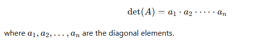
- Theorem: Determinant of a Triangular Matrix:
- The determinant of a triangular matrix (upper or lower) is the product of the diagonal elements.
- Cramer’s Rule:
These notes cover the essential concepts related to determinants and their properties. Understanding these properties and theorems is crucial for solving matrix-related problems in linear algebra, especially in areas like matrix inverses, systems of equations, and eigenvalues/eigenvectors.
13. Utility maximization and Profit Maximization Theorem
Exam Notes: Utility Maximization and Profit Maximization Theorem
1. Utility Maximization
Utility maximization refers to the process by which consumers allocate their income in such a way that they achieve the highest possible satisfaction or utility from the goods and services they consume. It is based on the assumption that consumers act rationally to maximize their well-being.
1.1 Utility Function
A utility function represents the relationship between the quantities of goods a consumer consumes and the level of satisfaction (or utility) derived from those goods.
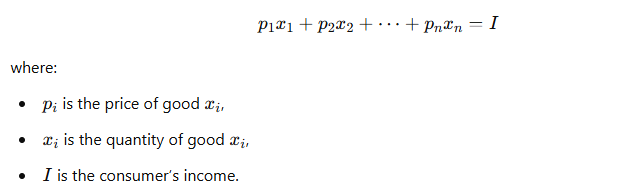
1.2 Budget Constraint
Consumers face a budget constraint because they have limited income, and they must decide how to allocate their income among different goods. The budget constraint is given by:
1.3 The Consumer’s Problem
To maximize utility, a consumer will choose the combination of goods that maximizes their utility function subject to their budget constraint.
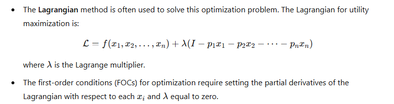
1.4 The Equimarginal Principle
The equimarginal principle states that consumers will allocate their income so that the ratio of marginal utility to price is the same for all goods:
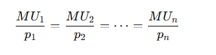
This ensures that the consumer is maximizing utility by equating the “bang for the buck” across all goods.
1.5 Conclusion: Utility Maximization
Consumers maximize utility when they allocate their income in such a way that the marginal utility per dollar spent on each good is equalized across all goods. The optimal consumption bundle can be found by solving the utility maximization problem subject to the budget constraint.
2. Profit Maximization Theorem
The Profit Maximization Theorem refers to the principle that firms aim to choose the level of output that maximizes their profit, which is the difference between total revenue and total cost. Profit maximization is a fundamental objective for firms in competitive markets.
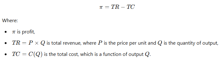
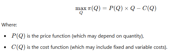
2.1 Profit Function
The profit function for a firm is the difference between its total revenue (TR) and total cost (TC):
2.2 Profit Maximization Problem
The firm’s goal is to choose the level of output QQ that maximizes profit. The firm’s profit maximization problem can be written as:
2.3 Marginal Revenue and Marginal Cost
To maximize profit, the firm will produce at the level where marginal revenue (MR) equals marginal cost (MC).
2.4 First-Order Condition for Profit Maximization
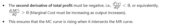
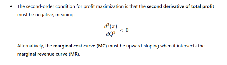
2.5 Second-Order Condition
To ensure that the solution is a maximum, the second derivative of the profit function with respect to QQ must be negative:
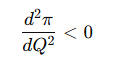
This guarantees that the function is concave and the firm is maximizing its profit.
2.6 Profit Maximization in Perfect Competition
In a perfectly competitive market, firms are price takers, meaning they cannot influence the market price. In this case:
- Price equals marginal cost: P=MC
- The firm maximizes profit by producing where marginal cost equals the market price.
2.7 Profit Maximization in Monopoly
In a monopoly, the firm has market power and can influence the price. The monopolist maximizes profit by setting marginal revenue equal to marginal cost: MR=MC
However, in a monopoly, marginal revenue is less than the price due to the downward-sloping demand curve.
3. Summary
- Utility Maximization:
- Consumers allocate their income to maximize utility, equating the marginal utility per dollar across all goods.
- The utility maximization problem is subject to the budget constraint, and the equimarginal principle guides the optimal consumption choice.
- Profit Maximization:
- Firms maximize profit by producing the quantity where marginal revenue equals marginal cost (MR=MC).
- In competitive markets, P=MC, while monopolists set MR=MC, but P>MC.
- The second-order condition ensures that the solution is a maximum.
Both utility maximization and profit maximization are fundamental concepts in microeconomics, representing consumer behavior and firm behavior, respectively.
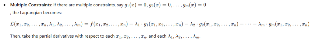
14. Lagrange multiplicity
Exam Notes: Lagrange Multipliers
1. Introduction to Lagrange Multipliers
The Lagrange multiplier method is a mathematical technique used for finding the local maxima and minima of a function subject to constraints. This method transforms a constrained optimization problem into an unconstrained optimization problem.
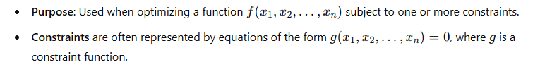
2. The Basic Concept
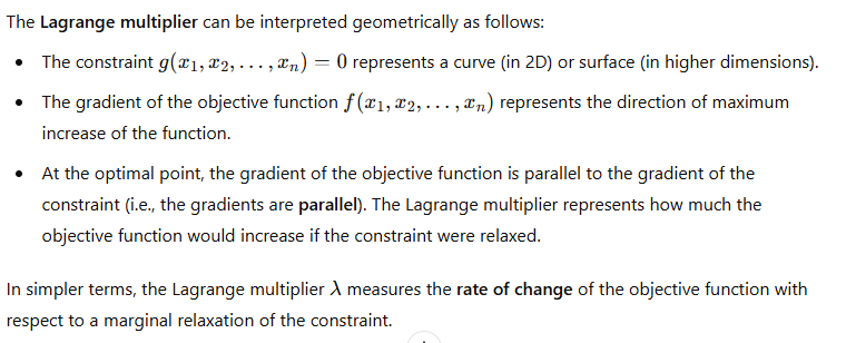
The Lagrange multiplier λ represents the sensitivity of the objective function to changes in the constraint. It measures how much the objective function will change if the constraint is relaxed by one unit.
3. Steps to Solve Using Lagrange Multipliers
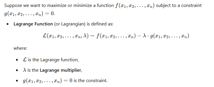
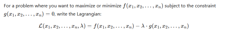
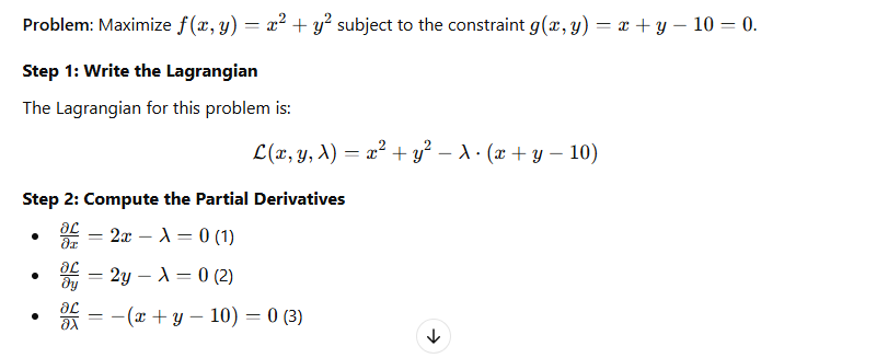
Step 1: Write the Lagrangian
Step 2: Compute Partial Derivatives
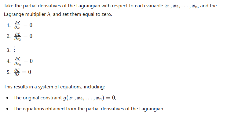
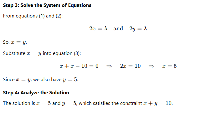
Step 3: Solve the System of Equations

Step 4: Analyze the Solution
- Verify if the critical points correspond to a maximum, minimum, or saddle point by using second-order conditions or by analyzing the behavior of the function.
4. Example of Lagrange Multiplier Method
5. Geometrical Interpretation of Lagrange Multipliers
The Lagrange multiplier can be interpreted geometrically as follows:
6. Second-Order Conditions
To confirm whether a point is a maximum or minimum, the second-order conditions can be used:
- Hessian Matrix: Compute the second-order partial derivatives of the Lagrangian with respect to the decision variables
- Positive Definite: If the Hessian is positive definite at the optimal point, it is a minimum.
- Negative Definite: If the Hessian is negative definite, it is a maximum.
7. Extensions of the Lagrange Multiplier Method
8. Conclusion
- The Lagrange multiplier method is a powerful tool for constrained optimization problems, allowing the transformation of constrained problems into simpler unconstrained ones.
- The Lagrange multiplier represents the rate at which the objective function changes as the constraint is relaxed.
- The method is widely used in economics, physics, and other fields for optimization problems with constraints.
15. Solution of linear programming problem by graphical method
Exam Notes: Solution of Linear Programming Problem by Graphical Method
1. Introduction to Linear Programming
Linear programming (LP) is a mathematical technique for optimizing (maximizing or minimizing) a linear objective function, subject to linear constraints. It is widely used in fields such as economics, business, engineering, and operations research to find the best outcome in decision-making problems.
1.1 Linear Programming Problem (LPP) Formulation
A standard Linear Programming Problem (LPP) is formulated as:
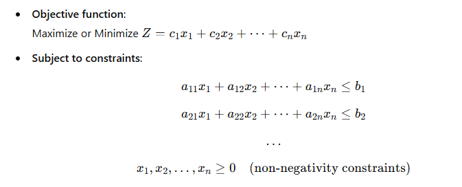
Where:
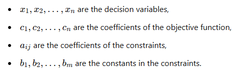
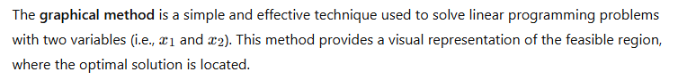
2. Graphical Method of Solving LPP
2.1 Steps for Solving an LPP by Graphical Method
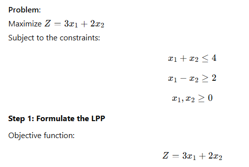
Step 1: Formulate the LPP
- Identify the objective function and constraints, and express them in standard form.
Step 2: Plot the Constraints
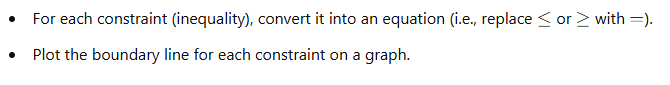
Step 3: Identify the Feasible Region
- The feasible region is the set of all points that satisfy all the constraints. This region is typically a polygon.
- The feasible region is bounded by the lines representing the constraints and the axes.
Step 4: Plot the Objective Function
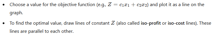
Step 5: Find the Optimal Solution
- The optimal solution occurs at one of the corner points (vertices) of the feasible region.
- To find the optimal value of the objective function, evaluate the objective function at each corner point.
- The corner point with the highest (or lowest) objective function value, depending on whether we are maximizing or minimizing, is the optimal solution.
Step 6: Check for Multiple or Infeasible Solutions
- If there are multiple corner points with the same value for the objective function, there may be infinitely many optimal solutions (i.e., the optimal solution lies along a line segment between those points).
- If no feasible region exists (the constraints are inconsistent), there is no solution to the problem.
3. Example of Solving a Linear Programming Problem by Graphical Method
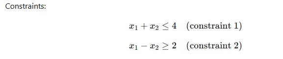
**Step to Plot the Constraints**
1. **Plot the constraint
**: – Find intercepts:
Plot the line connecting the points
2. **Plot the constraint
**: – Find intercepts:
Plot the line through the points
and extend it to find the feasible region.
3. **Non-negativity constraints
** – These represent the first quadrant, so the feasible region is confined to this part of the graph. **Step 3: Identify the Feasible Region** – The feasible region is the area that satisfies all the constraints. – It is the area where all the constraint lines overlap.
**Step for Plot the Objective Function**
Choose a value for
Rearrange this equation to get the intercepts: Draw the line passing through these intercepts.
#### **Step for Find the Optimal Solution
** – Move the objective function line parallel to itself, increasing the value of until it touches the furthest point in the feasible region. – The point where this happens is the optimal solution. For this problem, you will find that the optimal solution occurs at the verte
#### **Step 6: Check for Multiple or Infeasible Solutions** – In this case, there is a unique optimal solution at , so no further analysis is needed.
4. Key Points to Remember**
1. **Graphical method is limited to two variables**: –
The graphical method is practical only for solving LPPs involving two variables . – For more than two variables, other methods such as the **Simplex method** or **Interior-point methods** must be used.
2. **Feasible Region**: – The feasible region is bounded by the constraint lines and is the set of all points that satisfy all the constraints. – The optimal solution lies at one of the corner points (vertices) of this region.
3. **Objective Function**: – The objective function is maximized or minimized by evaluating it at each vertex of the feasible region. – The maximum (or minimum) value of the objective function will occur at one of the corner points.
4. **Multiple Optimal Solutions**: – If the objective function lines are parallel to the constraint boundary, there may be infinitely many optimal solutions along that line.
5. **Infeasible Solution**: – If no feasible region exists (the constraints are contradictory), there is no solution to the LPP.
5. Conclusion** The **graphical method** is an intuitive and effective way of solving linear programming problems with two variables. By graphing the constraints, identifying the feasible region, and evaluating the objective function at the corner points, the optimal solution can be easily determined. However, it is limited to two-variable problems and may not be applicable for more complex cases.
16. Input Output Analysis, Meaning, Analysis, Assumption, Transition, Technical Coefficient matrix and its solution
Exam Notes: Input-Output Analysis
1. Introduction to Input-Output Analysis
Input-Output Analysis is an economic model that represents the flow of goods and services in an economy. It focuses on how the production in one industry depends on the outputs of other industries. This method was developed by Wassily Leontief in the 1930s and is used to study the interrelations between different sectors of an economy, particularly for determining how changes in one sector can affect others.
2. Meaning of Input-Output Analysis
Input-Output analysis is a quantitative economic technique used to understand the relationships between industries or sectors of an economy. It looks at the interactions between industries by showing how the output of one industry is used as an input for another industry. This analysis is crucial for:
- Understanding inter-industry relationships in production.
- Analyzing the economic structure of an economy.
- Forecasting the economic impact of policy changes, investments, or technological advances.
3. Key Components of Input-Output Analysis
- Sectors/Industries: The economy is divided into different sectors (e.g., manufacturing, agriculture, services), and the analysis looks at how the output from one sector becomes an input for another.
- Input-Output Table: The table is the core of Input-Output analysis, showing the monetary flow of goods and services between industries.
- Final Demand: The final demand represents the goods and services that are consumed by households, the government, or exported to other countries.
4. Assumptions in Input-Output Analysis
The input-output model relies on several assumptions:
- Constant Coefficients: It assumes that the coefficients (i.e., the ratio of input required to produce one unit of output) remain constant, meaning the technological structure of the economy does not change over time.
- Linear Relationships: It assumes linear relationships between inputs and outputs. This means that if the production of one sector increases, the input required from other sectors will increase in a proportional manner.
- Closed System: The economy is treated as a closed system where all goods produced are used either as inputs for other goods or for final consumption (exports, government spending, etc.).
- No Substitution: The model assumes no substitution between goods. If one sector needs a particular input, it cannot substitute it with another input.
- No Supply Constraints: The model assumes that all inputs are available in sufficient quantities, meaning there are no supply constraints or resource limitations.
- Fixed Technology: The method assumes that the production technology of the economy remains unchanged over the time period under consideration.
5. Analysis in Input-Output
Input-Output analysis helps in the following ways:
- Inter-industry Relationships: It identifies how industries depend on each other and what is the role of each sector in the overall economy.
- Total Output Calculation: The model calculates the total output required in each sector to meet the demand, taking into account direct and indirect requirements.
- Economic Multiplier: The input-output model helps in calculating the economic multiplier effect — how an increase in one sector’s output affects the overall economy, including other sectors.
- Impact of Policy Changes: It can assess the effects of changes in government policies (e.g., investment in infrastructure, taxation) on various industries.
- Optimization: The analysis can be used to determine the most efficient allocation of resources and optimize production across sectors.
6. Transition Matrix in Input-Output Analysis
The transition matrix, often called the technical coefficient matrix, is a crucial part of input-output analysis. It represents the direct relationship between industries.
6.1 Definition of Transition Matrix
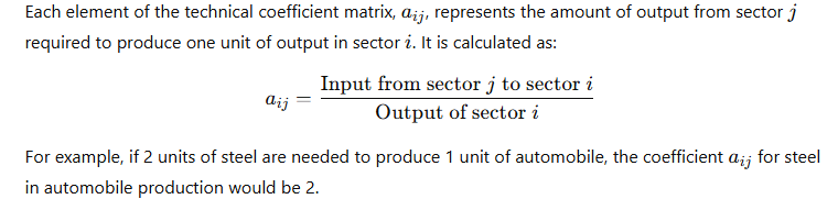
Let the input-output table consist of several industries, each represented by an output vector xx, and the intermediate demands are represented by a matrix AA. The transition matrix (also called the technical coefficient matrix) represents how much input from each sector is required to produce one unit of output in each sector.
Let:
Where:
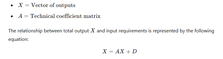
- A is the technical coefficient matrix, showing the direct inputs required by each sector to produce one unit of output.
- D is the final demand vector, showing the demand for goods and services from each sector.
- X is the total output vector, representing the total output of all industries.
6.2 Technical Coefficient Matrix
6.3 Importance of the Transition Matrix
- The transition matrix helps determine how changes in the final demand D affect the total output of the economy.
- It helps in understanding the relationships and dependencies between different sectors in the economy.
7. Solving the Input-Output Model
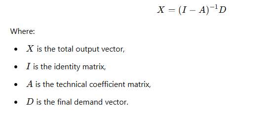
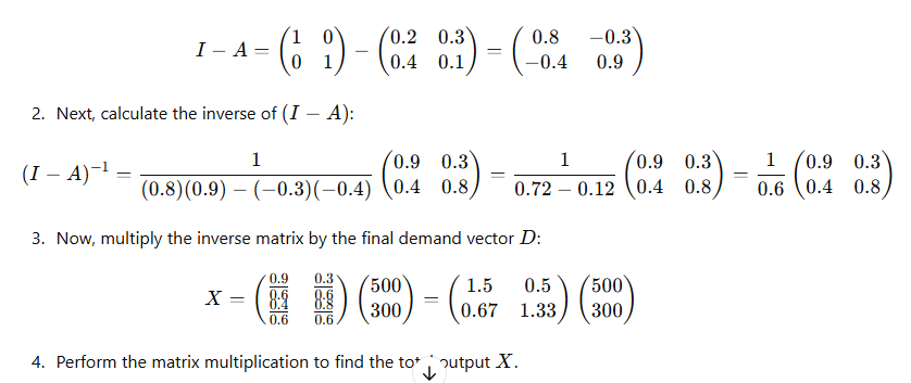
To solve an input-output model, we typically use the formula:
7.1 Steps to Solve the Input-Output Model
- Identify the Technical Coefficient Matrix (A): This matrix represents how much output from each industry is required to produce one unit of output in other industries.
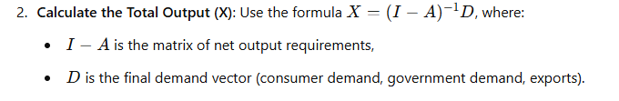
3. Interpret the Results: The resulting vector X gives the total output required from each sector to meet the demand.
7.2 Example
Suppose we have two sectors: Agriculture and Manufacturing. The technical coefficient matrix A is given as:
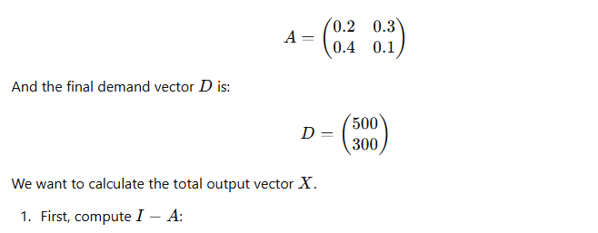
8. Conclusion
- Input-Output Analysis is a powerful method to understand the interrelationships between different sectors of an economy and to analyze the impact of changes in demand, investment, or policies.
- The transition matrix is central to input-output analysis, representing the technical coefficients that describe how sectors interact with each other.
- By solving the model using matrix algebra, we can determine the total output needed to meet final demand and study the economic structure more effectively.
17. Basic Concepts of Game Theory, Zero Sum Game, Non Zero Sum Game, Constant Sum Game, Game Strategy
Exam Notes: Game Theory and Its Concepts
1. Introduction to Game Theory
Game Theory is a mathematical framework used to analyze situations in which players (individuals, firms, countries, etc.) make decisions that are interdependent. The outcome for each player depends not only on their own choices but also on the choices made by others. Game theory is widely used in economics, political science, psychology, and strategic decision-making.
2. Basic Concepts of Game Theory
The key concepts in Game Theory include:
- Players: The decision-makers in the game (e.g., individuals, firms, countries).
- Strategies: A strategy is a plan of action that a player will follow, considering the possible choices available to them in the game. Strategies can be:
- Pure Strategy: A strategy where a player makes a specific choice and sticks to it.
- Mixed Strategy: A strategy where a player chooses among various options with certain probabilities.
- Payoffs: The rewards or outcomes that players receive from the game, which are typically represented in a payoff matrix.
- Equilibrium: A stable state of the game where no player has an incentive to deviate from their chosen strategy. The most famous equilibrium concept is the Nash Equilibrium.
- Nash Equilibrium: A situation where no player can improve their payoff by unilaterally changing their strategy, assuming the strategies of others remain unchanged.
3. Types of Games
Game theory divides games into several types based on the nature of the interactions between players. The most common types are:
3.1 Zero-Sum Game
- Definition: In a Zero-Sum Game, the total amount of reward (or “payoff”) in the game is constant. The gain of one player is exactly balanced by the loss of another player. The total payoff across all players always adds up to zero.
- Example: Poker is a classic example of a zero-sum game. The total money in the game remains constant, and if one player wins, they gain the amount lost by the other players.
- Key Features:
- One player’s gain is another player’s loss.
- Competitive in nature.
- The sum of the payoffs of all players is zero.
- Mathematical Representation: If Player A gains xx, Player B loses xx. The payoff matrix for a two-player zero-sum game will have the property that the row player’s gains will exactly offset the column player’s losses.
3.2 Non-Zero-Sum Game
- Definition: In a Non-Zero-Sum Game, the total payoff does not remain constant. The total payoff can vary, and the players’ gains or losses are not necessarily balanced. This allows for both players to potentially gain or both to lose.
- Example: Trade between two countries is a typical example of a non-zero-sum game. Both countries can gain from trade if they specialize in what they do best (comparative advantage).
- Key Features:
- Gains or losses are not strictly opposed.
- It is possible for both players to win or both players to lose.
- Cooperative strategies are often viable.
- Mathematical Representation: The payoffs for players can vary independently, and the sum of the payoffs does not equal zero.
3.3 Constant-Sum Game
- Definition: A Constant-Sum Game is a special case of a zero-sum game where the total payoff remains constant but may not necessarily equal zero. In other words, if one player wins or loses, the other player’s loss or gain is of the same magnitude but not necessarily zero.
- Example: A fixed division of a fixed prize (e.g., dividing $1000 between two players where one player gets $600 and the other gets $400).
- Key Features:
- The total payoff is constant, but it may not be zero.
- The sum of the payoffs for both players will always be the same.
- Mathematical Representation:

4. Game Strategy
In game theory, strategy refers to a complete plan of actions a player can take, considering the possible choices of the other players. The type of strategy chosen depends on the nature of the game (zero-sum, non-zero-sum, etc.).
4.1 Pure Strategy
- A Pure Strategy involves choosing one particular action or decision, without any randomness. The player always follows the same strategy regardless of the opponent’s moves.
- Example: In Rock, Paper, Scissors, a pure strategy might involve always choosing “rock”.
- Advantages:
- Simplicity.
- Clear predictability.
- Disadvantages:
- Can be easily exploited if the opponent knows the strategy.
4.2 Mixed Strategy
- A Mixed Strategy involves choosing among several possible actions with specific probabilities. This strategy is particularly useful in zero-sum games, where players may randomize their choices to avoid being predictable.

- Advantages:
- Helps in situations where players want to avoid being predictable.
- Disadvantages:
- Can be complex to analyze and implement.
4.3 Dominant Strategy
- A Dominant Strategy is one that results in a higher payoff for a player, regardless of the strategies chosen by the other players. If a player has a dominant strategy, they should choose it.
- Example: In a prisoner’s dilemma, confessing is a dominant strategy because, no matter what the other player does, it results in a better payoff for the player.
4.4 Nash Equilibrium and Strategy
- A Nash Equilibrium occurs when no player can improve their payoff by unilaterally changing their strategy, given the strategies of all other players. At the Nash equilibrium, every player is playing their best response to the other players’ strategies.
5. Examples of Games
5.1 Prisoner’s Dilemma
- Description: The Prisoner’s Dilemma is a non-zero-sum game where two players can either cooperate with each other or betray each other.
- Payoff Matrix:
| Cooperate | Betray | |
|---|---|---|
| Cooperate | -1, -1 | -3, 0 |
| Betray | 0, -3 | -2, -2 |
- Nash Equilibrium: Both players betray, even though both would be better off if they cooperated.
5.2 Battle of the Sexes
- Description: A situation where two players have different preferences for how they want to spend time, but both prefer to spend time together rather than apart.
- Payoff Matrix:
| Opera | Football | |
|---|---|---|
| Opera | 2, 1 | 0, 0 |
| Football | 0, 0 | 1, 2 |
- Nash Equilibrium: There are two equilibria: both go to the opera, or both go to football, depending on the coordination between the players.
6. Conclusion
- Game Theory is a powerful tool for analyzing strategic decision-making, used in economics, business, and political science.
- Different types of games, such as zero-sum, non-zero-sum, and constant-sum games, help model competitive or cooperative scenarios.
- Strategies can be pure or mixed, with concepts like dominant strategies and Nash Equilibrium helping to predict players’ optimal decisions.
Module 4:
Linear Programming Video: Watch Now