SEM2CC9: TMBU M.A ECONOMICS – STATISTICAL METHODS

Gyanodhan

2 months ago

Sampling and its Types
Skewness
Correlation
Simple Regression
Methods of constructing Index Number – problems in construction
Laspeyere, Paasche and Fishers index Number
Mathematical expectation
Hypothesis testing
Normal distribution
Probability
Time series
Statistics

1. Sampling and its Types

सैंपलिंग का अर्थ है किसी बड़ी जनसंख्या से एक छोटा समूह (नमूना) चुनना।

Here’s a concise, well-organized set of notes on Sampling and Its Types, tailored for M.A. Economics level students. These are suitable for study or class preparation:

Sampling and Its Types

M.A. Economics – Research Methodology Notes

1. Introduction to Sampling

Definition:
Sampling is the process of selecting a subset (sample) from a larger group (population) to estimate characteristics of the whole population.

Need for Sampling:

Economical and time-saving
More practical than a full census
Enables statistical inference
Useful in large-scale economic research, surveys, experiments

2. Key Concepts

Population: The entire group about which information is required.
Sample: A part of the population selected for analysis.
Sampling Frame: A list of all elements in the population.
Sampling Unit: The individual element or group considered for selection.
Parameter vs. Statistic:
- Parameter: A value that describes a characteristic of a population.
- Statistic: A value that describes a characteristic of a sample.

3. Types of Sampling

Sampling methods are broadly classified into:

A. Probability Sampling

(Based on random selection; every unit has a known, non-zero chance of selection)

a) Simple Random Sampling

Every member has an equal chance of being chosen.
Method: Lottery method, random number tables.
Use: When the population is homogeneous.

b) Systematic Sampling

c) Stratified Sampling

Population divided into strata (groups) based on characteristics (e.g. income, age), and random samples taken from each stratum.
Use: When population is heterogeneous.

d) Cluster Sampling

Population divided into clusters (usually geographic), and some clusters are selected randomly.
Use: When population is spread over large areas.

B. Non-Probability Sampling

(No random selection; some units may have zero chance of selection)

a) Convenience Sampling

Selection based on ease of access or availability.
Use: Exploratory research, pilot studies.

b) Judgmental/Purposive Sampling

Units selected based on researcher’s expertise or judgment.
Use: Expert surveys, case studies.

c) Snowball Sampling

Existing subjects recruit new participants from their contacts.
Use: Hidden or hard-to-reach populations (e.g., informal labor, drug users).

d) Quota Sampling

The population is divided into categories, and quotas are filled non-randomly.
Use: Market research, opinion polls.

4. Comparison Table

Criteria	Probability Sampling	Non-Probability Sampling
Selection Basis	Random	Non-random
Representativeness	High	Low
Bias	Low	High
Cost	Higher	Lower
Use in Economics	Surveys, experiments	Case studies, pilot studies

5. Importance in Economics

Essential for empirical research and policy formulation.
Used in national surveys (NSSO, NFHS), consumer behavior studies, income and employment analysis.
Enables estimation of population parameters with measurable accuracy.

Let me know if you’d like this as a downloadable PDF or formatted for presentation slides.

2. Skewness

डेटा वितरण के असंतुलन को मापता है:

Here are detailed and concise M.A. Economics-level notes on Skewness, including definitions, types, formulas, and examples, perfect for exams or class revision.

📘 Skewness

M.A. Economics – Statistical Methods / Quantitative Techniques Notes

🔹 1. Meaning of Skewness

Definition:
Skewness refers to the asymmetry or departure from symmetry in the distribution of data. A perfectly symmetrical distribution (like the normal distribution) has zero skewness.

Skewness tells us whether:

Most data values lie to the left or right of the mean.
The tail on one side of the distribution is longer than the other.

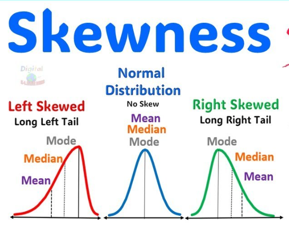
🔹 2. Types of Skewness

Type	Description	Relation (Mean, Median, Mode)	Diagram Shape
Symmetrical	Data is evenly distributed on both sides of the mean.	Mean = Median = Mode	Bell-shaped (Normal Distribution)
Positively Skewed	Tail is longer on the right side (high values).	Mean > Median > Mode	Peak to the left, tail to the right
Negatively Skewed	Tail is longer on the left side (low values).	Mean < Median < Mode	Peak to the right, tail to the left

🔹 3. Measures of Skewness

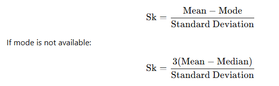
A. Karl Pearson’s Coefficient of Skewness

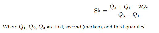
B. Bowley’s Coefficient of Skewness (based on quartiles)

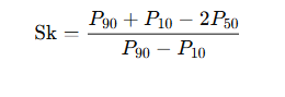
C. Kelly’s Coefficient of Skewness (based on percentiles or deciles)

🔹 4. Interpretation of Skewness

Sk > 0 → Positively skewed (right-skewed)
Sk < 0 → Negatively skewed (left-skewed)
Sk = 0 → Symmetrical

🔹 5. Example

Example 1: Using Pearson’s Method

Suppose in a sample:

Mean = 60
Median = 50
Standard deviation = 20

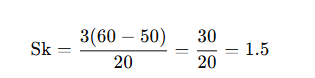
👉 Interpretation: The data is positively skewed, as the mean is greater than the median.

🔹 6. Importance of Skewness in Economics

Helps economists understand income distribution (e.g., skewed income in developing countries).
Useful in analyzing price distributions, wage structures, etc.
Important for policy design where average measures may be misleading.

📌 Quick Recap Table

Aspect	Positive Skew	Negative Skew	Symmetrical
Tail direction	Right	Left	Equal
Mean vs Median vs Mode	Mean > Median > Mode	Mean < Median < Mode	Mean = Median = Mode
Example	Wealth distribution	Exam scores (few failures)	Normal height distribution

3. Correlation

दो चरों के बीच रेखीय संबंध को मापता है:

Here are clear and concise M.A. Economics notes on Correlation, including definitions, types, methods, formulas, and a worked-out example.

📘 Correlation

M.A. Economics – Statistical Methods / Quantitative Techniques Notes

🔹 1. Meaning of Correlation

Definition:
Correlation is a statistical technique that measures the degree and direction of relationship between two or more variables.

For example: Studying the relationship between income and consumption, or education level and wage.

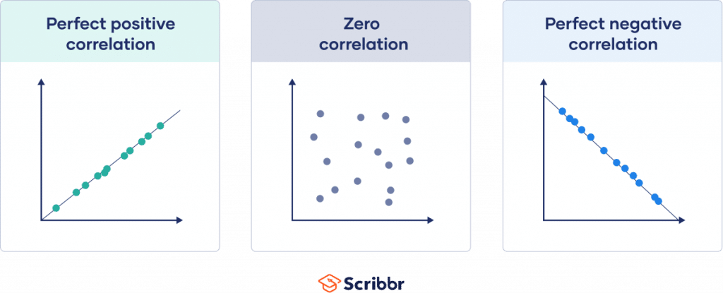
🔹 2. Key Concepts

Positive Correlation: Both variables increase or decrease together
e.g., Income ↑ → Consumption ↑
Negative Correlation: One variable increases, the other decreases
e.g., Price ↑ → Demand ↓
No Correlation: No consistent pattern between variables

🔹 3. Types of Correlation

Type	Explanation	Example
Positive Correlation	Variables move in the same direction	Income & Spending
Negative Correlation	Variables move in opposite directions	Price & Quantity Demanded
Perfect Correlation	Change in one variable leads to proportional change in another (r = ±1)	Celsius & Fahrenheit
Zero Correlation	No relationship (r = 0)	Shoe size & IQ

🔹 4. Methods of Measuring Correlation

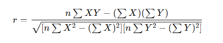
A. Karl Pearson’s Correlation Coefficient (r)

Measures the strength and direction of linear relationship.
Formula (for sample data):

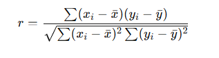
Range: −1 ≤ r ≤ +1
- r = +1 → Perfect positive correlation
- r = −1 → Perfect negative correlation
- r = 0 → No correlation

B. Spearman’s Rank Correlation (ρ)

Used for ranked or ordinal data.
Formula:

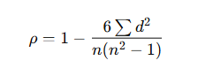
Where:

d = difference between ranks
n = number of observations

🔹 5. Example (Karl Pearson’s Method)

Let’s take data of 5 students:

Student	X (Study Hours)	Y (Marks)
A	2	30
B	4	50
C	6	65
D	8	80
E	10	95

Let’s use simplified Pearson’s formula:

Step 1: Calculate necessary values:

X	Y	XY	X²	Y²
2	30	60	4	900
4	50	200	16	2500
6	65	390	36	4225
8	80	640	64	6400
10	95	950	100	9025
Σ	Σ	Σ	Σ	Σ
30	320	2240	220	23050

Step 2: Plug into formula

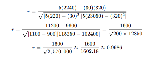
👉 Interpretation: Strong positive correlation between study hours and marks.

🔹 6. Importance of Correlation in Economics

Policy analysis: Understanding links between economic indicators (e.g., inflation and unemployment).
Forecasting: Predicting trends like demand based on income changes.
Economic modeling: Selecting relevant variables for regression analysis.
Market research: Studying consumer behavior relationships.

📌 Quick Recap Table

Measure	Use	Value Range	Data Type
Pearson’s r	Linear relationship between two variables	-1 to +1	Quantitative
Spearman’s ρ (rho)	Ranked or ordinal data	-1 to +1	Ordinal

4. Simple Regression

एक स्वतंत्र चर (X) के आधार पर आश्रित चर (Y) का अनुमान लगाना।

Here are clear and structured M.A. Economics-level notes on Simple Regression, suitable for class preparation, assignments, or exam revision.

📘 Simple Regression Analysis

M.A. Economics – Econometrics / Quantitative Techniques Notes

🔹 1. Introduction to Regression Analysis

Definition:
Regression analysis is a statistical tool used to study the relationship between a dependent variable and one or more independent variables.

In simple regression, we study the relationship between two variables:

Dependent variable (Y) – the variable we are trying to predict or explain.
Independent variable (X) – the variable used to explain Y.

Example: Predicting consumption (Y) based on income (X).

🔹 2. Purpose of Regression

Estimate the value of the dependent variable based on known values of the independent variable.
Understand the strength and direction of the relationship.
Test economic theories (e.g., Keynes’ consumption function).
Forecasting and prediction.

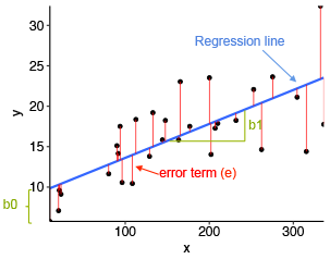
🔹 3. Simple Linear Regression Model

Model Equation:

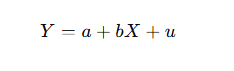
Where:

Y: Dependent variable
X: Independent variable
a: Intercept (value of Y when X = 0)
b: Slope (change in Y due to a one-unit change in X)
u: Error term (accounts for randomness or other factors not included)

🔹 4. Assumptions of the Classical Linear Regression Model (CLRM)

Linearity: Relationship between X and Y is linear.
Independence: Observations are independent.
Homoscedasticity: Constant variance of the error term.
No autocorrelation: Error terms are uncorrelated.
Normality: Errors are normally distributed.
No multicollinearity: (for multiple regression only)

🔹 5. Estimation: Ordinary Least Squares (OLS)

Objective: Minimize the sum of squared residuals

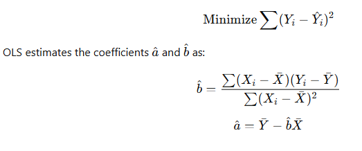
🔹 6. Example:

Suppose we have data:

Income (X)	Consumption (Y)
10	20
20	25
30	30
40	35
50	40

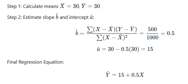
👉 Interpretation:

When income is 0, consumption is estimated at 15 (autonomous consumption).
For every 1 unit increase in income, consumption increases by 0.5 units.

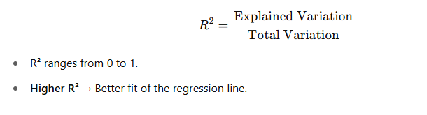
🔹 7. Goodness of Fit (R²)

🔹 8. Applications in Economics

Consumption and income analysis
Demand and price studies
Wage and education relationship
Investment and interest rate
Export and exchange rate modeling

🔹 9. Limitations of Simple Regression

Only two variables — may ignore other important factors
Assumes a linear relationship
Sensitive to outliers and missing variables
Cannot imply causation — only association

📌 Quick Recap Table

Component	Description
Dependent Variable (Y)	What we want to predict (e.g., consumption)
Independent Variable (X)	The cause or predictor (e.g., income)
Intercept (a)	Value of Y when X = 0
Slope (b)	Change in Y due to 1-unit change in X
R² (R-squared)	How well the model explains variation in Y

Let me know if you’d like:

A PDF version
A graphical illustration of regression line
Practice problems with solutions
I’m happy to help!

5. Methods of constructing Index Number – problems in construction

सूचकांक संख्याएँ समय के साथ परिवर्तनों को मापती हैं।

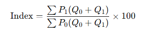
🔹 1. Meaning of Index Number

An Index Number is a statistical measure designed to show changes in a variable or group of related variables over time. It is often used to measure changes in prices, quantities, costs of living, wages, etc.

Example: Consumer Price Index (CPI), Wholesale Price Index (WPI)

🔹 2. Uses of Index Numbers in Economics

Measure inflation and deflation
Compare purchasing power of money over time
Assess changes in cost of living
Economic policy formulation
Trend analysis in production, trade, and employment

🔹 3. Methods of Constructing Index Numbers

There are two main types of index numbers:

Price Index Numbers
Quantity Index Numbers

✅ A. Simple (Unweighted) Index Numbers

i) Simple Aggregative Method

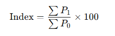
Where:

P1 = prices in current year
P0 = prices in base year

Limitations: All items are given equal importance regardless of their significance.

ii) Simple Average of Relatives Method

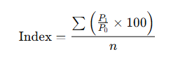
Where:

Each item’s price relative is calculated and then averaged.

✅ B. Weighted Index Numbers

Weights represent the relative importance of different items (e.g., quantity consumed).

i) Laspeyres’ Method (Base Year Weights)

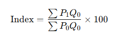
Uses base year quantities (Q₀) as weights
Tends to overstate price increase

ii) Paasche’s Method (Current Year Weights)

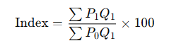
Uses current year quantities (Q₁)
Tends to understate price increase

iii) Fisher’s Ideal Index

Geometric mean of Laspeyres and Paasche
Satisfies both time reversal and factor reversal tests
Considered most ideal index

iv) Marshall-Edgeworth Index

Uses average of base and current year quantities as weights

🔹 4. Problems in Construction of Index Numbers

Constructing reliable and meaningful index numbers involves several difficulties:

A. Selection of Base Year

Should be a normal year (no war, pandemic, etc.)
If base year is not appropriate, the index will be misleading.

B. Choice of Items

Relevant and representative items must be selected.
Excluding key goods/services skews results.

C. Choice of Weights

Weights should reflect relative importance (consumption or production).
Inappropriate weights distort the index.

D. Price Quotations

Prices must be collected from reliable, consistent sources.
Variations in quality or location can cause errors.

E. Change in Quality

Over time, the quality of goods changes.
Difficult to adjust for improvements/deterioration.

F. Introduction of New Goods

New products enter the market (e.g., smartphones), which weren’t in the base year.
Makes comparisons difficult.

G. Obsolescence

Some goods become outdated and irrelevant (e.g., typewriters).

H. Time Factor

Long time gaps between current and base year reduce comparability.

🔹 5. Ideal Index Number – Desirable Qualities

Representativeness
Based on adequate data
Appropriate weights
Free from bias
Satisfies:
- Time reversal test
- Factor reversal test
- Circular test

📌 Summary Table of Methods

Method	Weights Used	Bias	Formula Type
Simple Aggregative	None	High	Total of current/base prices
Simple Relatives	None	High	Average of price relatives
Laspeyres	Base year quantities	Overstates inflation	∑P1Q0/∑P0Q0
Paasche	Current year quantities	Understates inflation	∑P1Q1/P1Q1
Fisher’s Ideal	Both	None (Ideal)	Geometric Mean

6. Laspeyere, Paasche and Fishers index Number

Laspeyres: आधार वर्ष की मात्रा पर आधारित।

Paasche: वर्तमान वर्ष की मात्रा पर आधारित।

Fisher: लैसपेयर और पास्चे का औसत।

Here is a clear and structured set of M.A. Economics notes on Laspeyres, Paasche, and Fisher’s Index Numbers, including definitions, formulas, interpretation, and a numerical example. These notes are suitable for assignments, exams, and presentations.

📘 Index Numbers: Laspeyres, Paasche, and Fisher’s Method

M.A. Economics – Statistical Methods / Price Index Numbers

🔹 1. Introduction to Index Numbers

An Index Number is a statistical measure that shows changes in a variable (e.g., prices, quantities) over time, usually in comparison to a base year.

Index numbers are widely used in price analysis, inflation measurement, cost of living studies, and economic planning.

🔹 2. Types of Weighted Index Numbers

We use weighted index numbers when we want to consider the relative importance (weights) of different items.

✅ A. Laspeyres Price Index

Formula:

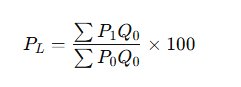
Where:

P1: Current year prices
P0: Base year prices
Q0: Base year quantities

Features:

Uses base year quantities as weights.
Easier to compute (data for current year prices and base year quantities are often available).

Limitation:

Tends to overstate price increases because it doesn’t account for changes in consumption patterns.

✅ B. Paasche Price Index

Formula:

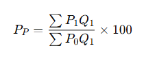
Where:

Q1: Current year quantities

Features:

Uses current year quantities as weights.
More realistic, as it reflects actual consumption in the current year.

Limitation:

Difficult to compute as current-year quantity data may not be available.
Tends to understate price increases.

✅ C. Fisher’s Ideal Price Index

Formula:

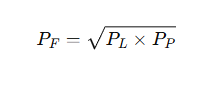
Features:

Geometric mean of Laspeyres and Paasche index numbers.
Considered most accurate and ideal.
Satisfies Time Reversal and Factor Reversal Tests (important tests for a good index).

📌 Comparison Table

Aspect	Laspeyres	Paasche	Fisher’s Ideal
Weights used	Base year quantities Q0	Current year quantities Q1	Both (geometric mean)
Bias	Overstates inflation	Understates inflation	No bias
Data requirement	Easier	Requires current data	Needs both sets of data
Accuracy	Moderate	Moderate	Highest
Satisfies Tests	No	No	Yes

🔹 3. Numerical Example

Let’s consider 2 commodities:

Commodity	P0	Q0	P1	Q1
A	10	5	12	6
B	8	10	10	12

✅ Step 1: Laspeyres Index

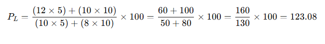
✅ Step 2: Paasche Index

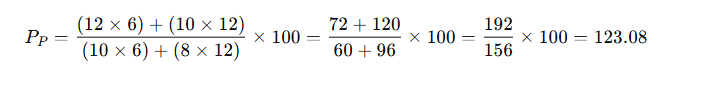
✅ Step 3: Fisher’s Index

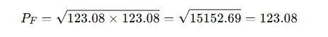
In this case, all three indices give the same result due to proportionate changes.

🔹 4. Interpretation

If index > 100 → Prices have increased compared to base year.
If index < 100 → Prices have decreased.
If index = 100 → No change in price level.

🔹 5. Importance in Economics

Laspeyres and Paasche methods form the basis for official indices like CPI and WPI.
Fisher’s method is used in academic and theoretical research due to its mathematical soundness.
These indices are essential for:
- Inflation targeting
- Wage adjustments
- Cost-of-living analysis
- Economic policy formulation

7. Mathematical expectation

कोई बात नहीं! आइए Mathematical Expectation (गणितीय आशा) को बहुत आसान हिंदी में समझते हैं।

🔷 Mathematical Expectation (गणितीय आशा) क्या है?

गणितीय आशा का मतलब है – किसी घटना से मिलने वाली औसत या अपेक्षित (expected) राशि या परिणाम।

यह बताया जाता है कि अगर कोई प्रयोग (experiment) बहुत बार दोहराया जाए, तो उसका औसतन परिणाम क्या होगा।

🔸 आसान भाषा में उदाहरण:

मान लीजिए कि एक सिक्का उछाला जा रहा है।

अगर हेड (Head) आए तो आप ₹10 जीतते हैं।
अगर टेल (Tail) आए तो आप ₹0 पाते हैं।

सवाल: इस गेम से मिलने वाली औसतन राशि (expected value) क्या है?

🔹 Step 1: संभावनाएँ (Probability)

हेड की संभावना = ½
टेल की संभावना = ½

🔹 Step 2: संभावित राशि × संभावना

हेड से मिलने वाली राशि = ₹10 × ½ = ₹5
टेल से मिलने वाली राशि = ₹0 × ½ = ₹0

🔹 Step 3: दोनों को जोड़ दो

Expected Value = ₹5 + ₹0 = ₹5

👉 यानी, इस गेम को बार-बार खेलने पर प्रति बार औसतन ₹5 मिलेंगे।

🔸 गणितीय सूत्र:

यदि किसी घटना में कई संभावित परिणाम हैं, तो:

🔸 एक और उदाहरण: पासा (Dice)

मान लो पासा फेंका गया। हर संख्या (1 से 6) की संभावना = 1/6

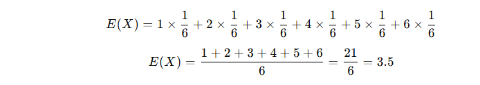
👉 यानी, पासा फेंकने पर औसतन संख्या 3.5 आएगी।

अगर आप चाहें, तो मैं इसके लिए चित्र (diagram), वीडियो लिंक या PDF नोट्स भी दे सकता हूँ।
क्या आप चाहेंगे कि इसे और उदाहरणों के साथ विस्तार से समझाया जाए?

Here are concise and well-structured M.A. Economics notes on Mathematical Expectation, suitable for exam preparation, assignments, or classroom reference.

📘 Mathematical Expectation (Expected Value)

M.A. Economics – Quantitative Techniques / Statistics

🔹 1. Meaning of Mathematical Expectation

Definition:
Mathematical Expectation (also known as Expected Value) is the average or mean value of a random variable over a large number of trials. It gives a measure of the central tendency of a probability distribution.

It is the value that one can expect on average if an experiment or process is repeated many times.

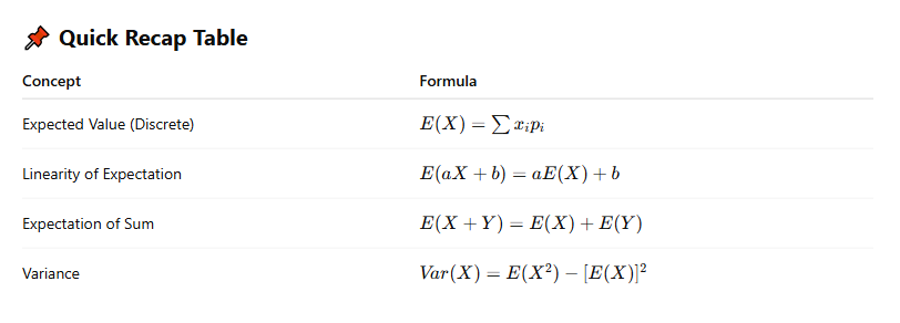
🔹 2. Notation and Formula

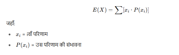
✅ For Discrete Variables:

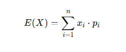
Where:

E(X): Expected value of X
xi: Possible outcome
pi: Probability of xi

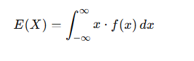
✅ For Continuous Variables:

If f(x)f(x)f(x) is a probability density function (PDF), then:

🔹 3. Properties of Mathematical Expectation

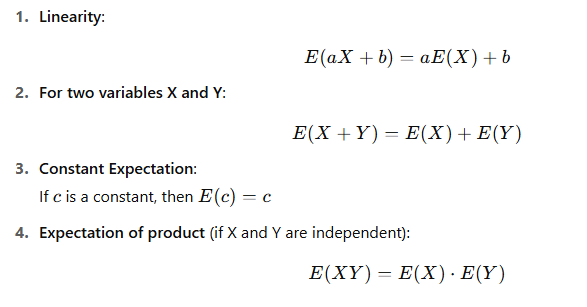
🔹 4. Economic Interpretation

In decision-making under uncertainty, expected value helps evaluate risky outcomes.
Expected utility theory uses E(X) to model consumer choices.
Helps in evaluating investment returns, insurance risks, and gambling outcomes.

🔹 5. Example – Discrete Case

A company is considering a new investment. The probabilities and returns are:

Profit (X in ₹ ‘000)	Probability (P)
10	0.1
20	0.3
30	0.4
40	0.2

👉 Interpretation: The expected profit is ₹27,000.

🔹 6. Variance and Standard Deviation (for context)

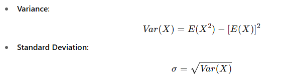
These measure the spread of the distribution around the expected value.

🔹 7. Applications in Economics

Cost-benefit analysis
Game theory and strategic decisions
Insurance and actuarial science
Portfolio theory and expected return on investment
Microeconomic theory – expected utility maximization

8. Hypothesis testing

सांख्यिकीय परिकल्पना को जांचने की प्रक्रिया।

कोई बात नहीं! आइए अब Hypothesis Testing (परिकल्पना परीक्षण) को बहुत सरल हिंदी में और स्टेप-बाय-स्टेप समझते हैं।

✅ Hypothesis Testing क्या है? (परिकल्पना परीक्षण)

जब हम कोई अनुमान या दावा (claim) करते हैं और यह जानना चाहते हैं कि वह सही है या नहीं — तब हम Hypothesis Testing करते हैं।

यह सांख्यिकी की एक प्रक्रिया है जिसमें हम यह जांचते हैं कि हमारा अनुमान (हाइपोथेसिस) सही है या नहीं।

🧠 आसान उदाहरण से समझिए:

मान लीजिए एक दवाई कंपनी कहती है कि उसकी दवा से 80% लोग ठीक हो जाते हैं।

अब आप यह जांचना चाहते हैं कि यह दावा सही है या नहीं।
यानी, कंपनी का दावा = एक परिकल्पना (Hypothesis) है।

🔍 Hypothesis Testing के मुख्य भाग:

1. Null Hypothesis (H₀)

यह कहता है कि “कोई बदलाव नहीं है”, “दावा सही है”
उदाहरण:
H₀: दवा 80% लोगों को ठीक करती है

2. Alternative Hypothesis (H₁ या Ha)

यह कहता है कि “दावा गलत हो सकता है”
उदाहरण:
H₁: दवा 80% से कम लोगों को ठीक करती है

✅ Hypothesis Testing करने के 5 Steps:

चरण	क्या करना है?	उदाहरण
1.	H₀ और H₁ तय करें	H₀: दवा असरदार है (80%) H₁: दवा असरदार नहीं है (80% से कम)
2.	Significance level (α) चुनें	आमतौर पर 0.05 यानी 5%
3.	Sample से डेटा लें और Test Statistic निकालें	जैसे Z-test या t-test
4.	Critical value से तुलना करें	Z > 1.96 तो H₀ को Reject
5.	फैसला लें	H₀ स्वीकार करें या अस्वीकार करें

🔺 2 Possible Result:

अगर H₀ सही है → हम उसे “स्वीकार” करते हैं।
अगर H₀ गलत है → हम उसे “Reject” करते हैं और H₁ को मानते हैं।

🔬 Common Tests:

Test	कब इस्तेमाल होता है
Z-Test	जब सैंपल बड़ा हो (n > 30) और मानक विचलन (standard deviation) ज्ञात हो
T-Test	जब सैंपल छोटा हो (n < 30) और मानक विचलन अज्ञात हो
Chi-Square Test	कैटेगोरिकल डेटा के लिए
ANOVA	एक से अधिक ग्रुप की तुलना करने के लिए

🧪 एक छोटा उदाहरण:

मान लीजिए एक स्कूल कहता है कि उसकी लड़कियाँ औसतन 70% नंबर लाती हैं। आप 10 लड़कियों का सैंपल लेते हैं और औसत निकलता है 65%, तो:

H₀: औसत = 70%
H₁: औसत ≠70%
फिर आप T-test करते हैं और देखते हैं कि क्या यह अंतर “महत्वपूर्ण” है या नहीं।

✨ आसान भाषा में निष्कर्ष:

बात	अर्थ
Hypothesis Testing	एक तरीका जिससे हम जांचते हैं कि कोई दावा सही है या नहीं
H₀	मूल परिकल्पना – “दावा सही है”
H₁	वैकल्पिक परिकल्पना – “दावा गलत हो सकता है”
Result	या तो H₀ को “स्वीकार” या “अस्वीकार” करना

क्या आप चाहेंगे कि मैं इसका वीडियो लिंक, पीडीएफ नोट्स, या एक एनिमेशन/चित्र से समझाऊँ?
या फिर किसी विशेष उदाहरण पर विस्तार से चलें?

Here is a well-structured and concise set of M.A. Economics notes on Hypothesis Testing, perfect for exam preparation or quick revision.

📘 Hypothesis Testing

M.A. Economics – Econometrics / Statistics

🔹 1. Introduction to Hypothesis Testing

Definition:
Hypothesis testing is a statistical procedure used to test whether a claim about a population parameter is true or false based on sample data. It helps in drawing conclusions about a population based on the sample evidence.

A hypothesis is a statement or claim about a population parameter (mean, proportion, variance, etc.).
Hypothesis testing involves formulating two competing hypotheses and using statistical methods to determine which hypothesis is supported by the data.

🔹 2. Types of Hypotheses

a) Null Hypothesis (H0):

The hypothesis to be tested.
It usually represents the idea that there is no effect or no difference.
Example: “The population mean is equal to 50.”

b) Alternative Hypothesis (H1 or Ha):

The opposite of the null hypothesis.
It represents the idea that there is an effect or difference.
Example: “The population mean is not equal to 50.”

🔹 3. Steps in Hypothesis Testing

Formulate Hypotheses:

Select a Significance Level (α\alphaα):

Choose the Appropriate Test:
- Z-test (for large sample sizes or when population variance is known)
- t-test (for small sample sizes or when population variance is unknown)
- Chi-square test, ANOVA, etc.
Compute the Test Statistic:
- Calculate the test statistic (e.g., Z-value, t-value) from the sample data.
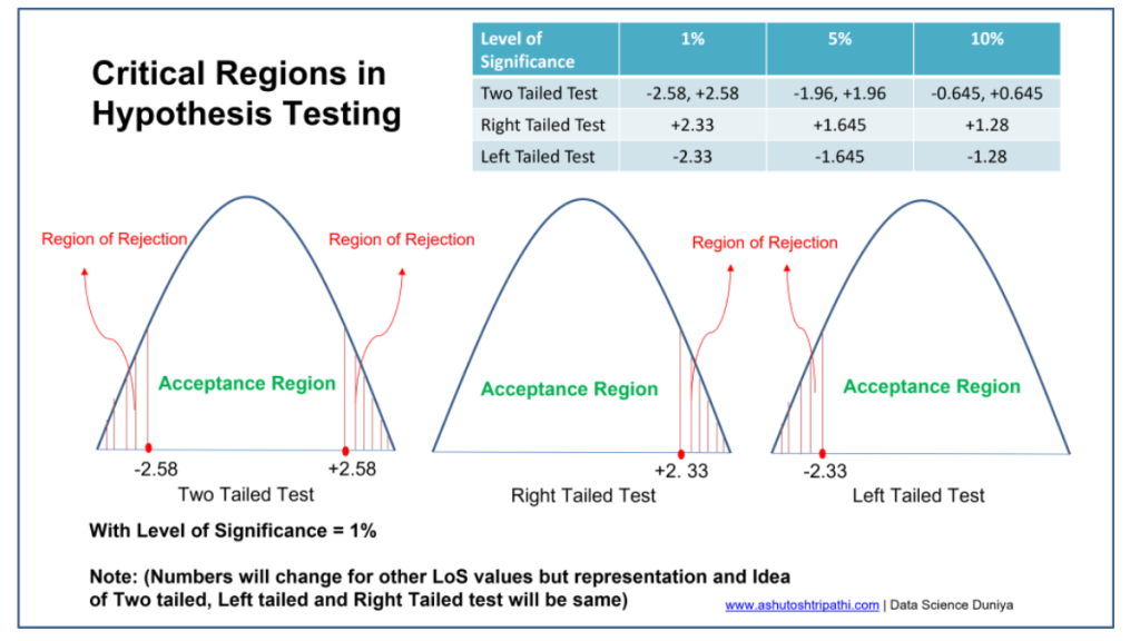
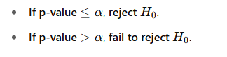
Make a Decision:
- Reject H0 if the test statistic falls within the critical region (i.e., the p-value is less than α\alphaα).
- Fail to reject H0 if the test statistic does not fall within the critical region.
Draw a Conclusion:
- Based on the test result, either reject the null hypothesis or fail to reject it.

🔹 4. Types of Errors in Hypothesis Testing

Type I Error (False Positive):
- Rejecting H0 when it is actually true.
- The probability of a Type I error is denoted by α\alphaα.
Type II Error (False Negative):
- Failing to reject H0 when it is actually false.
- The probability of a Type II error is denoted by β\betaβ.

🔹 5. Common Hypothesis Tests

a) Z-test (For large sample sizes or known population variance)

Used to test hypotheses about a population mean or proportion when the sample size is large (n>30n > 30n>30) or the population variance is known.

Formula for Z-test:

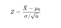
Where:

Xˉ\baˉ: Sample mean
μ0: Hypothesized population mean
σ: Population standard deviation
n: Sample size

b) t-test (For small sample sizes or unknown population variance)

Used when the sample size is small (n<30n < 30n<30) or when the population variance is unknown.

Formula for t-test:

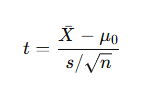
Where:

s: Sample standard deviation
Xˉ: Sample mean
μ0: Hypothesized population mean
n: Sample size

c) Chi-Square Test (For categorical data)

Used for testing goodness of fit, independence, and homogeneity of categorical data.

Formula for Chi-Square Test:

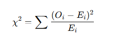
Where:

Oi: Observed frequency
Ei: Expected frequency

d) ANOVA (Analysis of Variance)

Used to test differences between more than two group means.

🔹 6. P-Value Approach

The p-value represents the probability of obtaining a result at least as extreme as the one observed, assuming the null hypothesis is true.

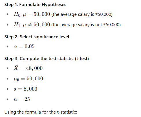
🔹 7. Example of Hypothesis Testing

Problem:
A company claims that the average salary of its employees is ₹50,000. A sample of 25 employees has an average salary of ₹48,000 with a standard deviation of ₹8,000. Test at the 5% significance level whether the company’s claim is true.

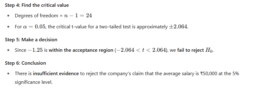
Step 6: Conclusion

There is insufficient evidence to reject the company’s claim that the average salary is ₹50,000 at the 5% significance level.

📌 Summary Table

Step	Action
1. Hypothesis Formulation	Null hypothesis H0, Alternative hypothesis H1
2. Significance Level (α\alphaα)	Common values: 0.05, 0.01
3. Test Statistic	Choose appropriate test (Z, t, Chi-square, etc.)
4. Critical Region	Determine critical value from table or p-value
5. Decision	Reject or fail to reject H0 based on test statistic
6. Conclusion	Final statement based on test results

9. Normal distribution

एक घंटी के आकार का संतुलित वितरण

Here are concise and clear notes on the Normal Distribution tailored for M.A. Economics students:

📘 Normal Distribution – Notes for M.A. Economics

1. Definition

A Normal Distribution is a continuous probability distribution that is symmetrical about its mean. Most of the observations cluster around the central peak, and the probabilities for values further away from the mean taper off equally in both directions.

2. Characteristics

Bell-shaped curve: Symmetric around the mean.
Mean = Median = Mode
Unimodal: One peak.
Asymptotic: The tails approach but never touch the horizontal axis.
Defined by two parameters:
- μ (mu) = Mean
- σ (sigma) = Standard deviation

3. Probability Density Function (PDF)

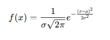
Where:

x is a value of the variable
μ\muμ is the mean
σ\sigmaσ is the standard deviation
e≈2.718e \approx 2.718e≈2.718

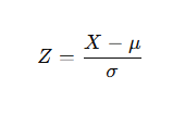
4. Standard Normal Distribution

A special case of the normal distribution where:

Mean μ=0
Standard deviation σ=1

Z-score transformation:

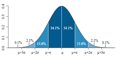
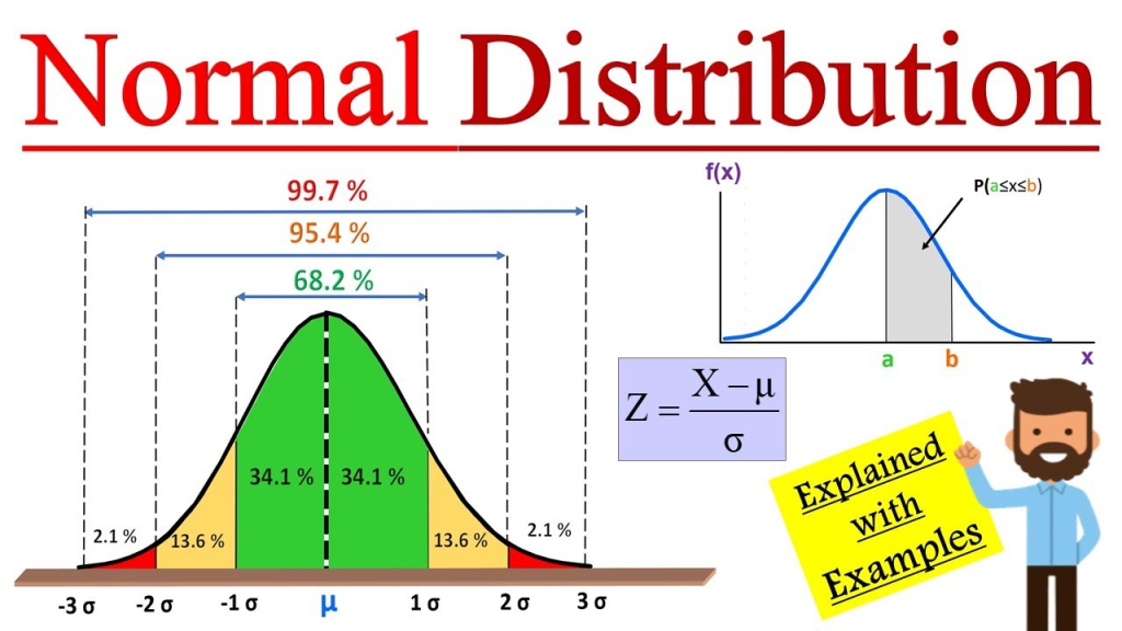
5. Empirical Rule (68–95–99.7 Rule)

In a normal distribution:

68% of data lies within 1σ
95% within 2σ
99.7% within 3σ

6. Applications in Economics

Forecasting and modeling (e.g., demand, prices, returns)
Hypothesis testing
Central Limit Theorem (sampling distributions approach normality)
Risk analysis and decision-making under uncertainty

7. Importance

Many economic variables approximate normality in large samples.
Useful in regression analysis, econometrics, and statistical inference.

10. Probability

किसी घटना के घटने की संभावना:

Here’s a structured and easy-to-understand version of Probability Notes tailored for M.A. Economics students:

📘 Probability – M.A. Economics Notes

1. Introduction to Probability

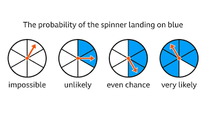
Probability is a numerical measure of uncertainty. It tells us how likely an event is to occur. It ranges from:

0 = impossible event
1 = certain event

2. Basic Terms

Term	Definition
Experiment	Any process or action that can produce some results (e.g. tossing a coin).
Sample Space (S)	The set of all possible outcomes of an experiment.
Event (E)	Any subset of a sample space (e.g. getting heads).
Outcome	A single possible result of an experiment.

3. Approaches to Probability

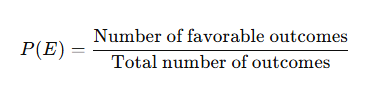
Classical / Theoretical

Based on logical reasoning.
Example: Tossing a fair coin.
Empirical / Statistical
Based on observed data or past records.
Subjective
Based on intuition, experience, or personal judgment.

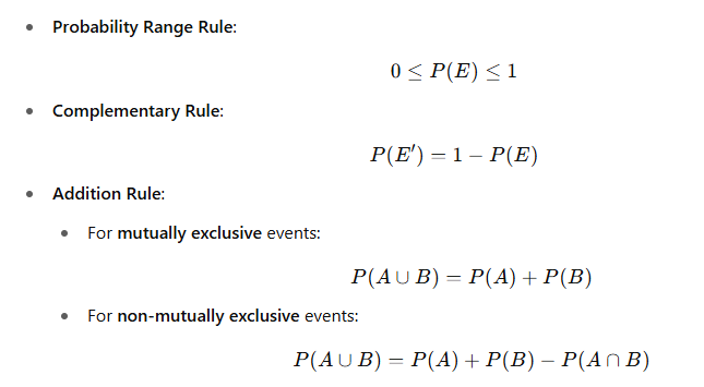
4. Rules of Probability

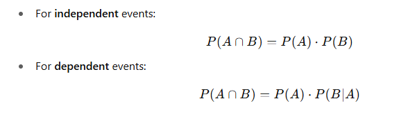
Multiplication Rule:

5. Conditional Probability

P(A∣B)=P(A∩B)P(B),if P(B)>0P(A|B) = \frac{P(A \cap B)}{P(B)}, \quad \text{if } P(B) > 0P(A∣B)=P(B)P(A∩B),if P(B)>0

It is the probability of A occurring given that B has occurred.

6. Bayes’ Theorem

P(A∣B)=P(B∣A)⋅P(A)P(B)P(A|B) = \frac{P(B|A) \cdot P(A)}{P(B)}P(A∣B)=P(B)P(B∣A)⋅P(A)

Used to revise probabilities in light of new evidence.

7. Random Variables

A random variable is a function that assigns a numerical value to each outcome of an experiment.

Discrete: Takes countable values (e.g. number of firms in a market).
Continuous: Takes any value in an interval (e.g. income, price).

8. Probability Distributions

Discrete Random Variable: Uses Probability Mass Function (PMF)
Continuous Random Variable: Uses Probability Density Function (PDF)
Cumulative Distribution Function (CDF): Gives the probability that a variable is less than or equal to a value.

9. Importance in Economics

Risk and uncertainty analysis
Consumer and firm behavior under uncertainty
Insurance and portfolio theory
Game theory and strategic decision-making
Econometric models (e.g., regression, maximum likelihood estimation)

✅ Summary

Concept	Formula/Key Point
Classical Probability	P(E)=FavorableTotalP(E) = \frac{Favorable}{Total}P(E)=TotalFavorable
Complement	P(E′)=1−P(E)P(E’) = 1 – P(E)P(E′)=1−P(E)
Addition Rule	P(A∪B)=P(A)+P(B)−P(A∩B)P(A \cup B) = P(A) + P(B) – P(A \cap B)P(A∪B)=P(A)+P(B)−P(A∩B)
Multiplication Rule	( P(A \cap B) = P(A) \cdot P(B
Conditional Probability	( P(A
Bayes’ Theorem	( P(A

11. Time series

समय के साथ एकत्रित आँकड़ों की श्रृंखला

Here are Time Series and Moving Average (M.A.) Notes in an Economics Context, tailored for students or professionals studying economic data.

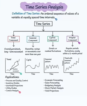
📘 TIME SERIES IN ECONOMICS

🔹 Definition:

A time series is a sequence of data points, typically economic indicators, measured over time at regular intervals (daily, monthly, quarterly, yearly).

🔹 Examples in Economics:

GDP growth rate (quarterly)
Inflation rate (monthly)
Unemployment rate (monthly)
Stock prices (daily)
Interest rates (monthly)

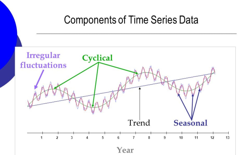
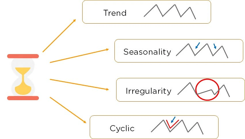
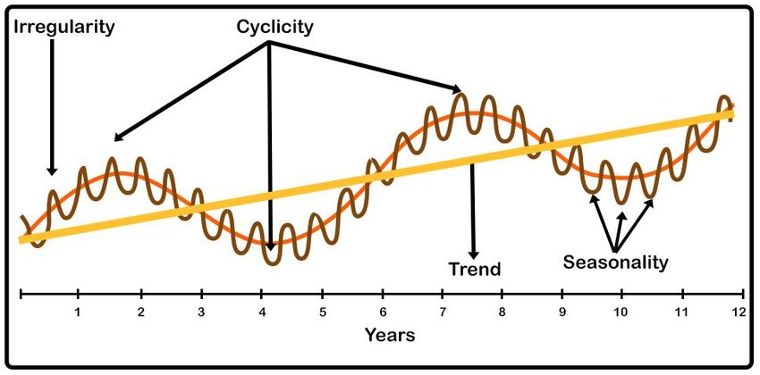
🧱 COMPONENTS OF TIME SERIES

Trend (T):
- Long-term increase or decrease in data.
- Reflects economic growth or decline (e.g., rising GDP over decades).
Seasonality (S):
- Regular pattern within a year due to seasons, policies, etc.
- Example: Higher retail sales in December (holiday season).
Cyclic Variation (C):
- Long-term economic cycles (e.g., business cycles).
- Periods of expansion and contraction (boom and recession).
Irregular/Random Variation (I):
- Unpredictable events (e.g., war, pandemic, natural disasters).

📉 MOVING AVERAGES (M.A.)

🔹 Purpose in Economics:

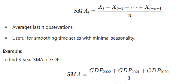
Smoothens short-term fluctuations in data.
Helps identify the underlying trend.
Used in forecasting and policy planning.

🔹 Types of Moving Averages:

1. Simple Moving Average (SMA):

2. Centered Moving Average (CMA):

Used when n is even (e.g., 4, 12).
Centers the average between two time periods.
Common in deseasonalizing economic data.

3. Weighted Moving Average (WMA):

Assigns higher weights to recent observations.
Better for detecting recent economic trends.

4. Exponential Moving Average (EMA):

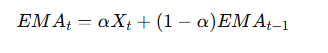
α\alphaα = smoothing constant (0 < α < 1)
More sensitive to recent changes in the economy.

🔍 USES IN ECONOMICS

Trend Analysis: Identifying long-term changes in economic indicators.
Forecasting: Predict future inflation, unemployment, etc.
Business Cycle Analysis: Understanding boom/recession phases.
Policy Evaluation: Helps governments and central banks analyze effects of policies over time.

📊 EXAMPLE TABLE

Year	GDP (₹ billion)	3-Year SMA
2020	2100	–
2021	2250	–
2022	2400	2250.00
2023	2600	2416.67
2024	2800	2600.00

📌 QUICK TIPS

Use odd-numbered M.A. for symmetric smoothing (3, 5, 7).
Use centered M.A. for seasonally adjusted data (e.g., 12-month).
For forecasting, M.A. gives short-term projections, while models like ARIMA give better long-term insights.

Internal Question: WHAT ARE THE COMPONENTS OF TIME SERIES

📌 कालक्रमिक श्रृंखला के घटक (Components of Time Series)

1️⃣ रुझान (Trend Component)

👉 समय के साथ-साथ डेटा में जो दीर्घकालिक बढ़ोतरी या गिरावट का पैटर्न दिखाई देता है, उसे रुझान कहते हैं।
📌 उदाहरण:
किसी कंपनी के सालाना बिक्री के आँकड़े में धीरे-धीरे वृद्धि होती जा रही है, जैसे:

2019 - ₹1,00,000  
2020 - ₹1,20,000  
2021 - ₹1,45,000  
2022 - ₹1,70,000

यहाँ पर बिक्री में लगातार वृद्धि का रुझान है।

2️⃣ मौसमी उतार-चढ़ाव (Seasonal Component)

👉 साल के एक ही समय पर बार-बार आने वाला उतार-चढ़ाव, जैसे तीज-त्योहार, मौसम आदि के कारण होता है।
📌 उदाहरण:
दुकानों में रक्षाबंधन या दिवाली के समय मिठाइयों की बिक्री का बढ़ जाना।

3️⃣ चक्रवातीय उतार-चढ़ाव (Cyclical Component)

👉 लम्बी अवधि में अर्थव्यवस्था में आए उतार-चढ़ाव, जैसे मंदी, उछाल आदि को चक्रवातीय उतार-चढ़ाव कहते हैं।
📌 उदाहरण:
COVID-19 महामारी के दौरान उद्योगों में गिरावट और फिर धीरे-धीरे रिकवरी का चक्र।

4️⃣ अनियमित घटक (Irregular/Random Component)

👉 आकस्मिक या अप्रत्याशित घटक जो अचानक और बिना पूर्व चेतावनी के आते हैं, जैसे आपदा, युद्ध, महामारी आदि।
📌 उदाहरण:
भूकंप के कारण कृषि उत्पादन में अचानक गिरावट।

📝 संक्षेप में (Summary Table):

क्रमांक	घटक	अर्थ	उदाहरण
1.	रुझान (Trend)	दीर्घकालीन वृद्धि/गिरावट	हर साल बढ़ती बिक्री
2.	मौसमी उतार-चढ़ाव (Seasonal)	हर साल एक ही समय पर उतार-चढ़ाव	त्योहारों पर बिक्री
3.	चक्रवातीय उतार-चढ़ाव (Cyclical)	अर्थव्यवस्था के उतार-चढ़ाव	मंदी और उछाल
4.	अनियमित घटक (Irregular)	अचानक अप्रत्याशित प्रभाव	भूकंप से नुकसान

📊 Components of Time Series

A time series is a sequence of data points recorded over time (e.g., daily, monthly, yearly). It is typically broken down into four main components:

1️⃣ Trend (T)

What is it?
The long-term movement in a time series—either upward, downward, or constant over time.
Example:
The steady increase in the average annual sales of a company over several years: 2019 - $100,000 2020 - $120,000 2021 - $140,000 2022 - $160,000 The sales are generally trending upward.

2️⃣ Seasonal Component (S)

What is it?
Regular, repeating short-term patterns within a fixed time period (like a year, month, or week).
Example:
Increased ice cream sales during summer months every year.

3️⃣ Cyclical Component (C)

What is it?
Long-term oscillations due to economic or business cycles (e.g., recession, boom), typically lasting longer than a year.
Example:
A company’s revenue decreasing during an economic downturn and increasing again during recovery.

4️⃣ Irregular (Random) Component (I)

What is it?
Unpredictable, random fluctuations due to unforeseen events (e.g., natural disasters, strikes).
Example:
A sudden drop in production due to a factory fire.

📝 Summary Table:

Component	What it Means	Example
Trend (T)	Long-term rise/fall	Annual sales growth
Seasonal (S)	Regular short-term patterns	Summer ice cream sales
Cyclical (C)	Long-term economic cycles	Business boom/recession
Irregular (I)	Random, unpredictable effects	Earthquake impact on agriculture

Details Me hai

📚 Time Series Components — Detailed Exam Notes

A time series is a sequence of observations recorded over time (e.g., daily, monthly, yearly). It can be decomposed into four main components:

1️⃣ Trend Component (T)

Definition:
The long-term movement in the data, showing the general direction (upward, downward, or stable) over a long period.

Characteristics:

Reflects persistent growth or decline.
Usually driven by factors like population growth, technological advancement, or long-term economic changes.

Example:

A company’s revenue steadily increasing over the years:
- 2018: $500,000
- 2019: $550,000
- 2020: $600,000
- 2021: $650,000
  This steady upward movement indicates a positive trend.

Note:
Trend is smooth, not affected by short-term fluctuations.

2️⃣ Seasonal Component (S)

Definition:
The regular, repeating short-term fluctuations within a year (or other time frame) caused by seasonal factors.

Characteristics:

Periodic and predictable.
Due to factors like climate, holidays, festivals, or cultural events.

Example:

Retail sales increase during Diwali or Christmas every year.
Tourist arrivals peak during summer or winter holidays.

Note:
Seasonal effects repeat in a fixed, known period, like quarterly, monthly, or weekly.

3️⃣ Cyclical Component (C)

Definition:
The long-term oscillations around the trend line, usually linked to business or economic cycles.

Characteristics:

Lasts longer than one year (often several years).
Caused by factors like economic booms, recessions, or global market changes.
Unlike seasonal variations, cyclical variations do not have a fixed, predictable period.

Example:

During a recession, sales may drop below the trend.
During an economic boom, sales may rise above the trend.

Note:
The cyclical component is irregular in length and amplitude compared to the seasonal component.

4️⃣ Irregular (Random) Component (I)

Definition:
Unpredictable, irregular variations caused by unforeseen events.

Characteristics:

Residual fluctuations that cannot be explained by trend, seasonal, or cyclical factors.
Often due to natural disasters, strikes, wars, pandemics, etc.

Example:

A sudden flood disrupts agricultural production.
COVID-19 pandemic causing abrupt changes in sales and production.

Note:
These are non-repetitive and unpredictable.

📌 Summary Table:

Component	Meaning	Timeframe	Examples
Trend (T)	Long-term direction (rise/fall)	Years	Steady increase in sales
Seasonal (S)	Regular, repeating fluctuations	Within a year	Festival sales, summer ice-cream sales
Cyclical (C)	Business/economic cycles	Several years	Recession impact on jobs
Irregular (I)	Unpredictable shocks	Unpredictable	Earthquake disrupting supply

✍️ Additional Points for Exams:

✅ Trend + Seasonal + Cyclical + Irregular components together explain the observed time series.
✅ Mathematically:

Time Series = T + S + C + I   (Additive model)
or
Time Series = T × S × C × I  (Multiplicative model)

✅ The model choice (additive/multiplicative) depends on data characteristics.

12. Statistics

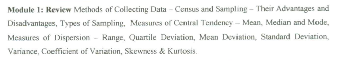
यहाँ Module 1: Review में दिए गए सभी विषयों की हिन्दी में सरल व्याख्या दी गई है:

1. डेटा एकत्र करने की विधियाँ (Methods of Collecting Data)

जनगणना (Census):
जब पूरी आबादी से जानकारी एकत्र की जाती है।
✅ लाभ: सटीक परिणाम
❌ हानि: समय और पैसा ज़्यादा लगता है
सैम्पलिंग (Sampling):
आबादी के एक छोटे हिस्से (सैंपल) से जानकारी इकट्ठा की जाती है।
✅ लाभ: समय और लागत कम
❌ हानि: यदि नमूना ठीक से न लिया जाए तो गलत निष्कर्ष निकल सकता है
सैम्पलिंग के प्रकार (Types of Sampling):
जैसे कि सरल यादृच्छिक सैम्पलिंग (Simple Random Sampling), स्तरीकरण सैम्पलिंग (Stratified), क्लस्टर सैम्पलिंग (Cluster Sampling) आदि।

2. केंद्रीय प्रवृत्ति के माप (Measures of Central Tendency)

माध्य (Mean):
सभी संख्याओं का औसत
👉 सूत्र: (सभी मानों का योग) ÷ (कुल संख्या)
माध्यिका (Median):
व्यवस्थित आंकड़ों में मध्य का मान
बहुलक (Mode):
सबसे अधिक बार आने वाला मान

3. प्रसरण के माप (Measures of Dispersion)

रेंज (Range):
अधिकतम और न्यूनतम मान का अंतर
👉 सूत्र: अधिकतम – न्यूनतम
चतुर्थांश विचलन (Quartile Deviation):
👉 Q3 और Q1 के बीच का आधा अंतर
👉 सूत्र: (Q3 – Q1) / 2
माध्य विचलन (Mean Deviation):
औसत से सभी मानों की औसत दूरी
मानक विचलन (Standard Deviation):
यह मापता है कि डेटा औसत से कितना दूर फैला हुआ है
प्रसरण (Variance):
मानक विचलन का वर्ग
👉 सूत्र: SD²
प्रसरण गुणांक (Coefficient of Variation – CV):
👉 सूत्र: (SD / Mean) × 100
तुलना के लिए उपयोगी

4. विकृति (Skewness)

यह बताता है कि वितरण संतुलित है या नहीं।
- Positive Skewed: पूंछ दाईं ओर लंबी होती है
- Negative Skewed: पूंछ बाईं ओर लंबी होती है

5. कुर्टोसिस (Kurtosis)

यह वितरण के चोटी (peak) की तीव्रता को दर्शाता है:
- Leptokurtic: बहुत तीखी चोटी
- Mesokurtic: सामान्य
- Platykurtic: समतल चोटी

यहाँ Module 2: Review के सभी टॉपिक्स की हिन्दी में व्याख्या दी गई है:

1. सहसंबंध की संकल्पना (Concept of Correlation)

यह दो चरों (variables) के बीच संबंध को दर्शाता है — जैसे कि X और Y।
सहसंबंध यह बताता है कि यदि एक चर बढ़ता है तो क्या दूसरा भी बढ़ता है या घटता है।

2. कार्ल पीयरसन का सहसंबंध गुणांक (Karl Pearson’s Coefficient of Correlation)

यह सांख्यिकीय सूत्र द्वारा निकाला जाता है।
मान: -1 ≤ r ≤ +1
- r = +1: पूर्ण सकारात्मक सहसंबंध
- r = -1: पूर्ण नकारात्मक सहसंबंध
- r = 0: कोई सहसंबंध नहीं

👉 सूत्र: r=∑(x−xˉ)(y−yˉ)∑(x−xˉ)2∑(y−yˉ)2r = \frac{\sum (x – \bar{x})(y – \bar{y})}{\sqrt{\sum (x – \bar{x})^2 \sum (y – \bar{y})^2}}

3. स्पीयरमैन का रैंक सहसंबंध (Spearman’s Rank Correlation Coefficient)

यह रैंक किए गए डेटा के लिए उपयोगी होता है (जब संख्यात्मक नहीं बल्कि रैंक होता है)।
👉 सूत्र:

ρ=1−6∑d2n(n2−1)\rho = 1 – \frac{6 \sum d^2}{n(n^2 – 1)}

जहाँ d=d = रैंकों का अंतर

4. आंशिक एवं गुणक सहसंबंध (Partial and Multiple Correlation)

Partial Correlation:
जब दो चरों के बीच सहसंबंध निकाला जाता है और बाकी चर स्थिर माने जाते हैं।
Multiple Correlation:
जब एक चर का संबंध दो या अधिक स्वतंत्र चरों के साथ देखा जाता है।
👉 उदाहरण: Y का X1 और X2 के साथ संबंध

5. सरल प्रतिगमन (Simple Regression)

यह एक निर्भर चर (Dependent Variable) और एक स्वतंत्र चर (Independent Variable) के बीच संबंध को बताता है।
👉 रूप:

Y=a+bXY = a + bX

जहाँ:

Y = निर्भर चर
X = स्वतंत्र चर
a = प्रतिच्छेदन (intercept)
b = ढाल (slope / regression coefficient)

6. प्रतिगमन गुणांकों का अनुमान (Estimation of Regression Coefficients)

सबसे सामान्य तरीका है: लीस्ट स्क्वेयर विधि (Method of Least Squares)
यह विधि उस रेखा को ढूंढती है जो त्रुटियों (errors) का वर्गीय योग (sum of squared errors) न्यूनतम करता है।

यहाँ Module 3: Review में दिए गए सभी विषयों की हिन्दी में व्याख्या दी गई है:

1. सूचकांक संख्याओं का निर्माण एवं उपयोग (Methods of Constructing Index Numbers and Their Uses)

सूचकांक संख्याएँ (Index Numbers):
यह सांख्यिकीय उपकरण होते हैं जो समय के साथ किसी वस्तु या सेवा की कीमतों, मात्रा या अन्य मूल्यों में परिवर्तन को मापते हैं।
उपयोग:
- महंगाई को मापने के लिए
- आर्थिक विश्लेषण
- सरकार की नीतियों का मूल्यांकन

2. भारित सूचकांक (Weighted Index)

इसमें हर वस्तु या सेवा को उसके महत्व (वजन) के अनुसार महत्व दिया जाता है।
इससे अधिक सटीक मापन होता है।

3. विभिन्न सूचकांक विधियाँ (Laspeyres, Paasche, Fisher Indices)

a. लैसपेयर सूचकांक (Laspeyres Index)

बेस ईयर (आधार वर्ष) की मात्रा को स्थिर मानकर बनाया जाता है।
👉 सूत्र:

L=∑(P1⋅Q0)∑(P0⋅Q0)×100L = \frac{\sum (P_1 \cdot Q_0)}{\sum (P_0 \cdot Q_0)} \times 100

b. पास्शे सूचकांक (Paasche Index)

वर्तमान वर्ष की मात्रा को आधार बनाता है।
👉 सूत्र:

P=∑(P1⋅Q1)∑(P0⋅Q1)×100P = \frac{\sum (P_1 \cdot Q_1)}{\sum (P_0 \cdot Q_1)} \times 100

c. फिशर सूचकांक (Fisher’s Ideal Index)

Laspeyres और Paasche दोनों का औसत होता है, और इसे “आदर्श सूचकांक” कहा जाता है।
👉 सूत्र:

F=L×PF = \sqrt{L \times P}

4. जीवन यापन लागत सूचकांक (Cost of Living Index Numbers)

यह सूचकांक मापता है कि किसी विशेष समूह के लिए वस्तुओं और सेवाओं की कीमतों में कितनी वृद्धि हुई है।
इसका उपयोग वेतन संशोधन, महंगाई भत्ते आदि के लिए किया जाता है।

अगर आप किसी एक विधि या सूत्र को उदाहरण सहित समझना चाहते हैं, तो मुझे बताइए!

यहाँ Module 4: Probability (प्रायिकता) से संबंधित सभी विषयों की हिन्दी में सरल व्याख्या दी गई है:

1. प्रायिकता की संकल्पना (Concept of Probability)

यह गणना करता है कि किसी घटना के घटने की संभावना कितनी है।

2. प्रायिकता की परिभाषाएँ (Definitions of Probability)

शास्त्रीय परिभाषा (Classical):
सभी संभावित परिणाम समान रूप से संभव हों।
👉 सूत्र: P(E)=सफल परिणामों की संख्यासंभावित परिणामों की कुल संख्याP(E) = \frac{\text{सफल परिणामों की संख्या}}{\text{संभावित परिणामों की कुल संख्या}}
अनुभवजन्य परिभाषा (Empirical):
प्रयोग या अनुभवों पर आधारित — जितनी बार घटना घटी / कुल प्रयोगों की संख्या

3. योग और गुणा के नियम (Laws of Addition and Multiplication)

योग का नियम (Addition Rule): P(A∪B)=P(A)+P(B)−P(A∩B)P(A \cup B) = P(A) + P(B) – P(A \cap B)
गुणा का नियम (Multiplication Rule): P(A∩B)=P(A)⋅P(B∣A)P(A \cap B) = P(A) \cdot P(B|A)

4. सशर्त प्रायिकता और बेयेस प्रमेय (Conditional Probability & Bayes’ Theorem)

सशर्त प्रायिकता (Conditional Probability):
किसी घटना की संभावना, जब कोई दूसरी घटना पहले ही घट चुकी हो।
👉 सूत्र: P(A∣B)=P(A∩B)P(B)P(A|B) = \frac{P(A \cap B)}{P(B)}
बेयेस प्रमेय (Bayes’ Theorem):
पुराने ज्ञान को अपडेट करने के लिए उपयोग किया जाता है।
👉 सूत्र: P(A∣B)=P(B∣A)⋅P(A)P(B)P(A|B) = \frac{P(B|A) \cdot P(A)}{P(B)}

5. गणितीय अपेक्षा (Mathematical Expectation)

यह एक यादृच्छिक चर का औसत मान होता है।
👉 सूत्र: E(X)=∑P(x)⋅xE(X) = \sum P(x) \cdot x

6. वितरण (Distributions)

a. बाइनोमियल वितरण (Binomial Distribution):

जब केवल दो संभावित परिणाम होते हैं: सफलता और असफलता
👉 उदाहरण: सिक्का उछालना

b. पॉइसन वितरण (Poisson Distribution):

जब घटनाएँ किसी निश्चित समय या स्थान में घटती हैं, और वे स्वतंत्र होती हैं।
👉 उदाहरण: 1 घंटे में आने वाली कॉल्स की संख्या

c. सामान्य वितरण (Normal Distribution):

घंटी-आकार का ग्राफ (Bell-Shaped Curve)
बहुत सामान्य रूप से इस्तेमाल होने वाला वितरण है

7. सामान्य वितरण के गुण (Properties of Normal Distribution)

मध्यमान (Mean), माध्यिका (Median), और बहुलक (Mode) तीनों समान होते हैं
वक्र समानुपाती (Symmetrical) होता है
क्षेत्रफल का 68%, 95% और 99.7% क्रमशः 1, 2 और 3 मानक विचलनों के भीतर होता है

यहाँ Module 5 के सभी विषयों की हिन्दी में संक्षिप्त और स्पष्ट व्याख्या दी गई है:

1. अनुमानक और उसका सैम्पल वितरण (Estimator and Its Sampling Distribution)

अनुमानक (Estimator):
वह सूत्र या नियम जिससे हम किसी जनसंख्या (Population) का माप, सैम्पल (नमूना) से अनुमान लगाते हैं।
उदाहरण: xˉ\bar{x} (सैम्पल का औसत) जनसंख्या के औसत μ\mu का अनुमानक है।
Sampling Distribution:
किसी अनुमानक की बार-बार सैम्पल लेकर बनी वितरण।

2. एक अच्छे अनुमानक के गुण (Desirable Properties of a Good Estimator)

अविकंपीता (Unbiasedness): अनुमान सही हो
संगति (Consistency): सैम्पल साइज बढ़े तो अनुमान सही के और पास आए
क्षमताशीलता (Efficiency): न्यूनतम वेरिएंस हो
पर्याप्तता (Sufficiency): सैम्पल से ज्यादा जानकारी मिले

3. सांख्यिकीय परिकल्पना का निर्माण (Formulation of Statistical Hypotheses)

शून्य परिकल्पना (Null Hypothesis, H₀): कोई अंतर या प्रभाव नहीं है
वैकल्पिक परिकल्पना (Alternative Hypothesis, H₁): अंतर या प्रभाव है

4. त्रुटियों के प्रकार (Types of Errors)

Type I Error:
H₀ सत्य होते हुए भी उसे गलत मान लेना
Type II Error:
H₀ झूठा होते हुए भी उसे सही मान लेना

5. परिकल्पना परीक्षण (Testing of Hypothesis)

जनसंख्या के औसत का परीक्षण (Testing Mean from Large Sample):
- Z-test का उपयोग करते हैं जब सैम्पल बड़ा हो (n > 30)
- तुलना करते हैं कि xˉ\bar{x} और μ\mu में कोई फर्क है या नहीं
दो जनसंख्याओं के औसत का अंतर (Difference between Means of Two Populations):
- Z-test या t-test द्वारा तुलना की जाती है

6. विभिन्न परीक्षण विधियाँ (Use of Z, t, Chi-square, and F distributions)

Z-test:
जब सैम्पल बड़ा हो और मानक विचलन ज्ञात हो
t-test:
जब सैम्पल छोटा हो (n < 30) और σ अज्ञात हो
Chi-square test (χ²):
- Independence या goodness of fit को जाँचने के लिए
- श्रेणियों पर आधारित डेटा के लिए प्रयोग होता है
F-test:
- दो वेरिएंस की तुलना के लिए
- ANOVA में उपयोग होता है

यदि आप किसी विशेष परीक्षण (जैसे Z-test या Chi-square) का उदाहरण और विस्तार से तरीका जानना चाहें, तो मुझे बताइए!

यहाँ Module 6 के सभी विषयों की हिन्दी में सरल व्याख्या दी गई है:

📘 Module 6: Time Series Analysis (समय श्रंखला विश्लेषण)

1. समय श्रंखला विश्लेषण (Time Series Analysis)

समय के अनुसार व्यवस्थित आंकड़ों (data) का विश्लेषण
उद्देश्य: भविष्य की प्रवृत्तियों (trend), मौसमी प्रभाव आदि को समझना और पूर्वानुमान लगाना।

2. समय श्रंखला के घटक (Components of Time-Series Data)

समय श्रंखला में मुख्यतः चार घटक होते हैं:

Secular Trend (दीर्घकालीन प्रवृत्ति):
- लम्बे समय में डेटा का स्थायी बदलाव (जैसे जनसंख्या में वृद्धि)
Seasonal Variation (मौसमी भिन्नता):
- मौसम, तीज-त्योहार, आदि से उत्पन्न होने वाले नियमित उतार-चढ़ाव
Cyclical Variation (चक्रीय भिन्नता):
- व्यापार चक्र जैसे मंदी, तेजी इत्यादि जो लंबे समय में दोहराते हैं
Irregular Variation (अनियमित भिन्नता):
- प्राकृतिक आपदा, युद्ध, महामारी जैसे अप्रत्याशित कारणों से हुआ बदलाव

3. दीर्घकालीन प्रवृत्ति की पहचान (Determination of Secular Trend)

i) मूविंग एवरेज विधि (Moving Average Method):

डेटा को ‘स्मूथ’ करके दीर्घकालीन प्रवृत्ति का पता लगाया जाता है
उदाहरण: 3-वर्षीय मूविंग एवरेज = वर्ष 1 + वर्ष 2 + वर्ष 33\frac{\text{वर्ष 1 + वर्ष 2 + वर्ष 3}}{3}

ii) साधारण न्यूनतम वर्ग विधि (Ordinary Least Square Method):

गणितीय समीकरण (जैसे: Y=a+bxY = a + bx) के माध्यम से trend निकालते हैं
इसमें ‘a’ intercept होता है और ‘b’ slope (ढाल) दर्शाता है

यदि आप किसी विधि (जैसे Moving Average या Least Squares) को उदाहरण सहित विस्तार से समझना चाहें, तो कृपया बताइए — मैं समाधान सहित समझाऊँगा।