Objective Question with Solution
Objective Question:
GEORGE B. DANTZIG: – Linear Programming
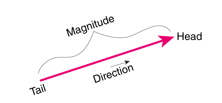
A vector Includes:- Magnitude and Direction
Transpose of Column Matrix is:- Row Matrix
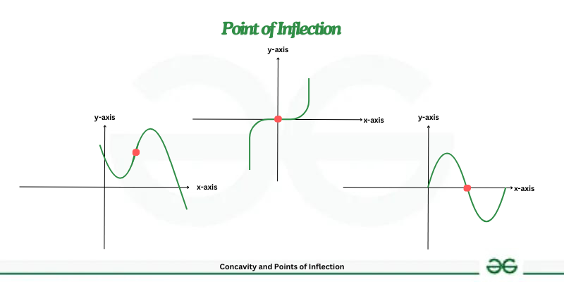
Point of inflation:- A function neither represent maximum value nor minimum value
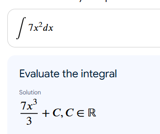
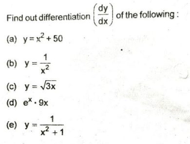
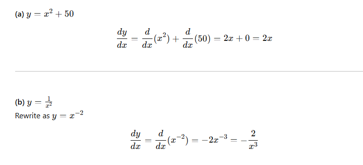
x^4, dy/dx= 4x^3
y= 3x+3 is explicit function

Input output technique was invented by = Wassily Leontief
The derivative of a constant function is zero
As we know that a square matrix in which all the principal diagonal elements are equal to 1 and rest of the elements are zero is called an identity matrix.
The slope of the demand curve is negative.
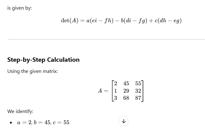
Determinant of 5 4
-9 3 is 51
Short Answer Type Questions with Answer:
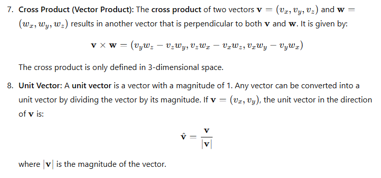
1. What is vector? Explain its properties
What is a Vector?
A vector is a mathematical object that has both magnitude (size) and direction. Vectors are used to represent quantities that require both magnitude and direction, such as displacement, velocity, force, and acceleration. Vectors are typically represented as arrows in a graphical sense, where the length of the arrow represents the magnitude and the direction of the arrow represents the direction.
Representation of a Vector:
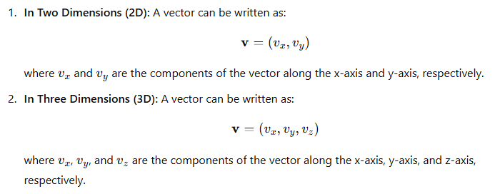
3. Graphically: Vectors can be represented as arrows. The direction of the vector is indicated by the direction of the arrow, and the length represents the magnitude.
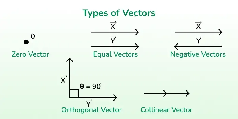
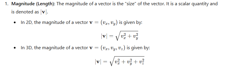
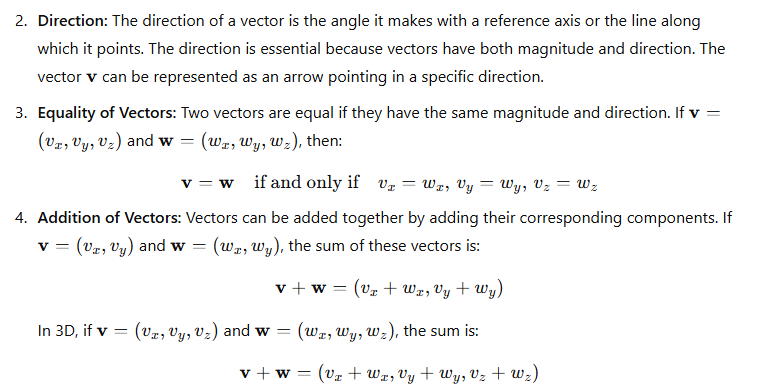
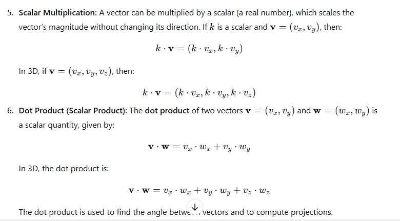
Properties of Vectors:
Conclusion:
A vector is a quantity that has both magnitude and direction, and it is used to represent many physical quantities like force, velocity, and displacement. Key properties of vectors include their ability to be added, multiplied by scalars, and to have dot and cross products.
2. Explain the relationship between TR, AR and MR
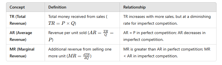
The relationship between Total Revenue (TR), Average Revenue (AR), and Marginal Revenue (MR) is fundamental to understanding how a firm’s revenue changes with respect to the quantity of goods sold and the price at which they are sold.
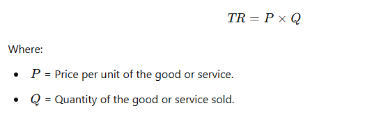
1. Total Revenue (TR):
Total Revenue (TR) is the total amount of money a firm receives from selling its goods or services. It is calculated as the price per unit (P) multiplied by the quantity sold (Q):
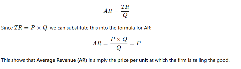
2. Average Revenue (AR):
Average Revenue (AR) is the revenue per unit of output sold. It is defined as:
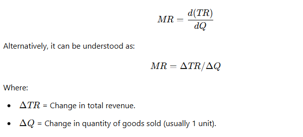
3. Marginal Revenue (MR):
Marginal Revenue (MR) is the change in Total Revenue resulting from the sale of one more unit of output. It is the derivative of Total Revenue (TR) with respect to quantity (Q):
Relationship Between TR, AR, and MR:
- AR and Price:
- From the formula AR = P, we can see that Average Revenue (AR) is the price of the good or service, assuming the firm is selling the good at a constant price. If the price changes (for example, in imperfect competition), AR will change as well.
- MR and TR:
- Marginal Revenue (MR) represents how total revenue changes as the firm sells one more unit. If MR is greater than zero, the firm’s total revenue is increasing. If MR is negative, total revenue is decreasing.
- Relationship Between AR and MR:
- For perfect competition, AR = MR = P, since the firm is a price taker and the price remains constant as quantity changes.
- For monopoly or imperfect competition, MR is generally less than AR. This is because, in these markets, the firm must lower the price to sell more units, which means that the marginal revenue from selling additional units decreases. As a result, MR declines faster than AR.
- In monopoly, the MR curve lies below the AR curve (or demand curve) because the firm must reduce the price to sell additional units, and this price reduction applies to all previous units sold, not just the additional units.
- Graphical Relationship:
- Total Revenue (TR) curve typically has an upward-sloping shape at first (as quantity increases) but can start to flatten or even decline at higher levels of output.
- Average Revenue (AR) is the price per unit, which often equals the demand curve for the firm.
- Marginal Revenue (MR) curve typically starts above the AR curve (for imperfect competition) but slopes downward faster than AR, especially for monopolistic firms.
Key Points:
- For a perfectly competitive firm:
- AR=MR= P.
- The firm’s total revenue increases at a constant rate as more units are sold.
- For a monopolistic or imperfectly competitive firm:
- AR is greater than MR because to sell more units, the firm has to lower the price, affecting the revenue of all units sold, not just the additional ones.
Summary of Relationships:
Conclusion:
- In perfect competition, AR and MR are equal and constant (since price is constant).
- In imperfect competition, MR is less than AR and declines faster than AR as output increases, due to the need to reduce the price to sell more units.
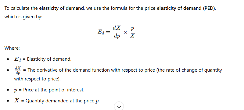
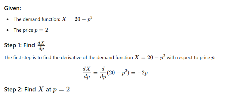
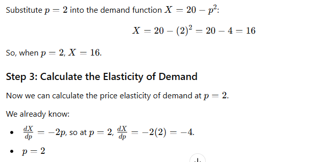
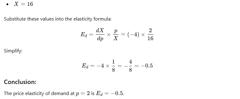
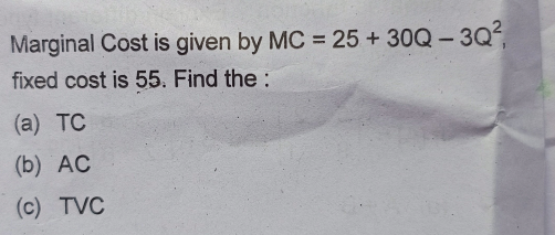
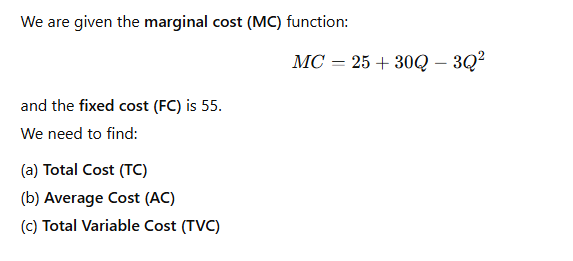
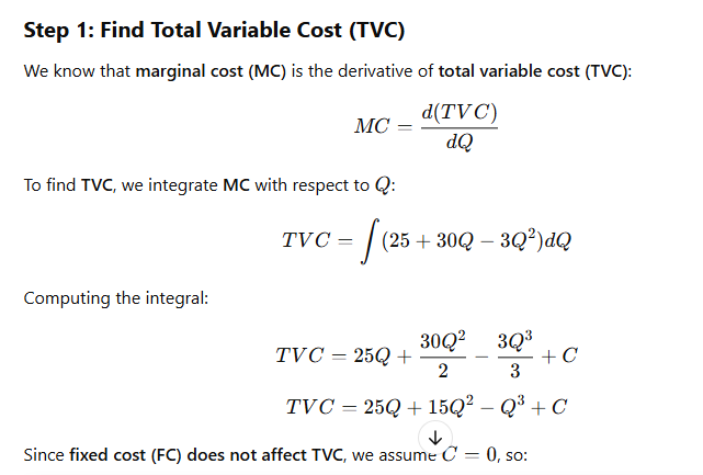
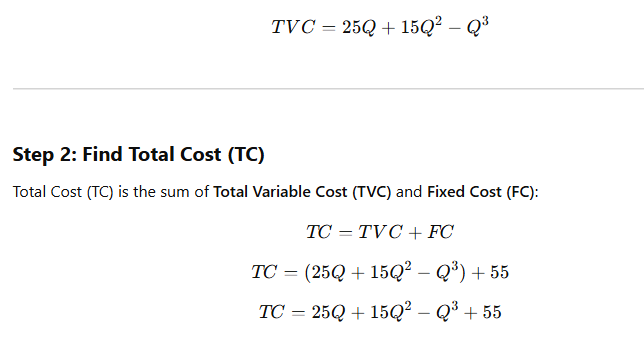
3. If demand function is X=20-p^2 and p=2 then find out elasticity of demand

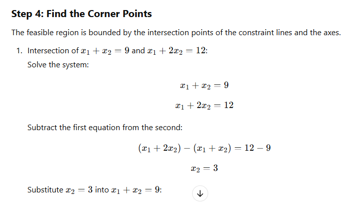
Feasible Region in Linear Programming
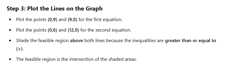
In linear programming, the feasible region is the set of all possible solutions that satisfy the given constraints of the problem. It is typically represented as a shaded area on a graph where all inequalities overlap.
Key Characteristics:
- Defined by Constraints: The feasible region is formed by the intersection of all linear inequalities (constraints) in the problem.
- Closed and Bounded: In many cases, the feasible region is a polygon that is closed and limited in size, but it can also be unbounded in some situations.
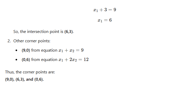
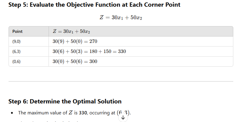
- Contains Optimal Solutions: The optimal solution (maximum or minimum value) for the objective function will always be found at a vertex (corner point) of the feasible region, if a solution exists.
- No Solution Region: If the constraints do not overlap or intersect in a meaningful way, the feasible region may be empty, indicating no valid solution exists.
Example:
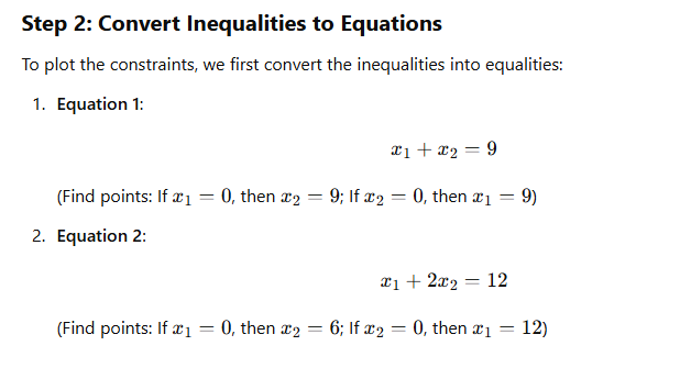
If the constraints are:
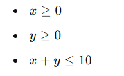
The feasible region will be the area within these boundary conditions.
In short, the feasible region plays a crucial role in identifying the possible solutions and locating the optimal point in linear programming problems.
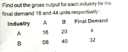
Hawkins-Simon Conditions in Input-Output Analysis
The Hawkins-Simon conditions are essential criteria used in input-output analysis to ensure the feasibility and stability of an economic system.
Key Points:
- Purpose: These conditions determine whether a given input-output system can achieve a viable production solution with positive outputs.
- Matrix Condition: The Hawkins-Simon condition states that for the input-output model to have a feasible non-negative solution:
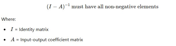
3. Economic Interpretation: The condition ensures that the economy’s production process is capable of meeting its internal and external demands without resulting in negative outputs.
4. Practical Importance: The Hawkins-Simon condition is crucial in ensuring that the production structure is sustainable and that resource requirements are balanced effectively.
In summary, the Hawkins-Simon conditions provide a mathematical framework to assess the stability and viability of an input-output economic model, ensuring realistic and positive production outcomes.

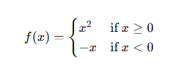
What is a Function?
A function is a mathematical relation that maps each element from a set called the domain to exactly one element in another set called the codomain. In simpler terms, a function defines a rule that assigns one output for every valid input.
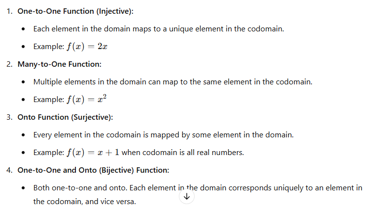
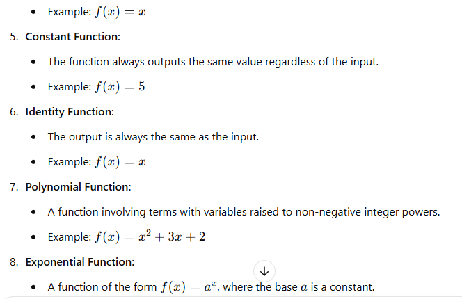
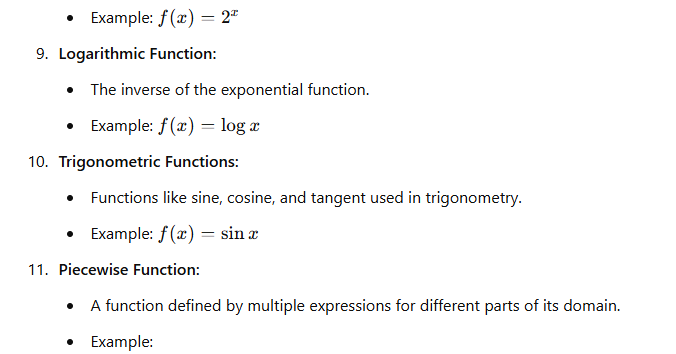
Types of Functions
Functions can be categorized into various types based on their properties:
Conclusion
Functions are fundamental in mathematics, modeling relationships in various fields such as science, engineering, and economics. Understanding different types of functions helps in solving diverse mathematical problems.

Zero-Sum or Constant-Sum Game
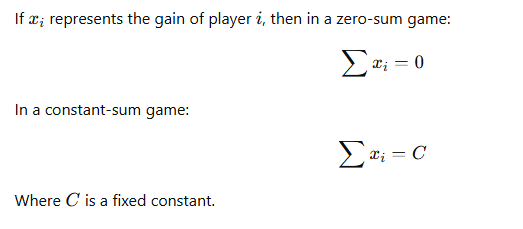
A zero-sum game (or constant-sum game) is a concept in game theory where the total gain or loss among all participants is always zero (or a fixed constant).
Key Characteristics:
- Fixed Total Payoff:
- In a zero-sum game, one player’s gain is exactly equal to another player’s loss.
- The total sum of outcomes for all players remains constant, often zero.
- Competitive Nature:
- These games are purely competitive, meaning players are in direct opposition.
- Strategic Decision-Making:
- Each player aims to maximize their own benefit while minimizing the opponent’s gain.
Mathematical Representation:
Examples:
- Chess: One player’s victory is the other player’s defeat.
- Poker: The total amount of money won by some players is equal to the total amount lost by others.
- Bidding in Auctions: The seller’s gain equals the buyer’s loss (in terms of extra spending).
Conclusion:
Zero-sum and constant-sum games are crucial in economic theory, competitive strategy, and decision-making models. They highlight the importance of strategic planning and understanding opponent moves.
Concept of Consumer’s Surplus and Producer’s Surplus
(a) Consumer’s Surplus
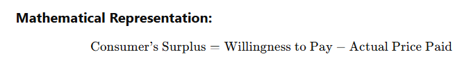
Consumer’s surplus is the difference between what consumers are willing to pay for a good or service and what they actually pay. It reflects the extra benefit consumers receive when they pay less than their maximum willingness to pay.
Mathematical Representation:
Example:
If a consumer is willing to pay ₹100 for a product but buys it for ₹70, the consumer surplus is ₹30.
(b) Producer’s Surplus
Producer’s surplus is the difference between what producers actually receive for a good or service and the minimum amount they are willing to accept. It represents the additional benefit producers gain from selling at a price higher than their minimum acceptable price.
Mathematical Representation:

Example:
If a producer is willing to sell a product for ₹50 but sells it for ₹70, the producer surplus is ₹20.
Graphical Interpretation:
- Consumer surplus is represented by the area above the market price and below the demand curve.
- Producer surplus is represented by the area below the market price and above the supply curve.
Both concepts are essential in understanding market efficiency, welfare economics, and the benefits consumers and producers derive from market transactions.
LONG ANSWER TYPE QUESTION
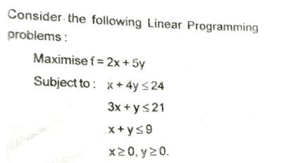
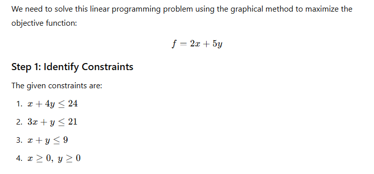
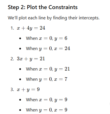

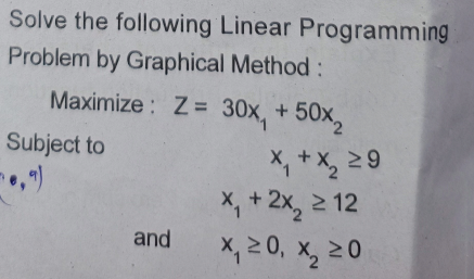
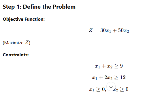
What is Linear Programming?
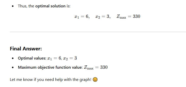
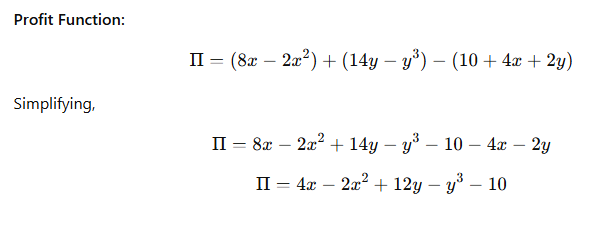
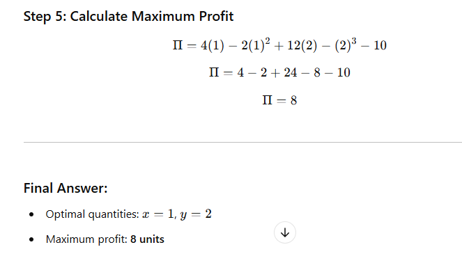
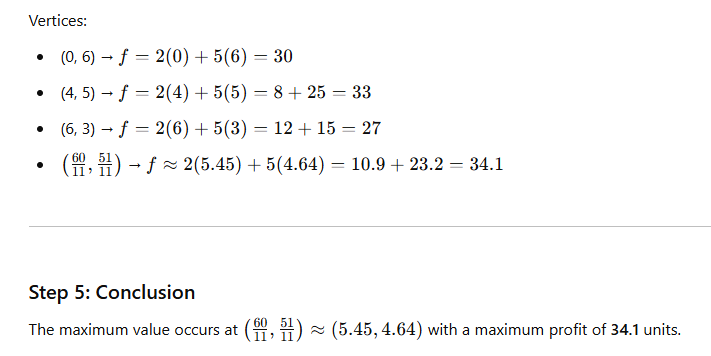
Linear Programming (LP) is a mathematical technique used to optimize a given objective function, subject to a set of linear constraints. It is widely used in decision-making to maximize profit or minimize cost while considering available resources and limitations.
Assumptions of Linear Programming
- Linearity – The relationships between decision variables are linear, meaning both the objective function and constraints are linear equations.
- Additivity – The total effect of all decision variables is the sum of their individual contributions.
- Divisibility – Decision variables can take fractional values, meaning they are continuous rather than discrete.
- Certainty – All coefficients in the objective function and constraints are known and constant.
- Non-Negativity – Decision variables cannot be negative, meaning all values must be zero or positive.
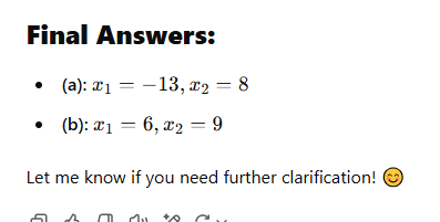
Let me know if you need further clarification! 😊